Simulating Network Diffusion with R

Cheng-Jun Wang
06/03/2014

Introduction

In this talk, I present how to simulate the most simple network diffusion with R. The algorithm is quite simple:

  • Generate a network g: g(V, E).
  • Randomly select one or n nodes as seeds.
  • Each infected node influences its neighbors with probability p (transmission rate, β).

SI model

Actually, this is the most basic epidemic model (SI model) with only two states: Susceptible (S) and Infected (I)! However, we will extend it to networks. Given the transmission rate \( \beta \), SI model can be described as:

\( \frac{dS}{dt}=-\beta SI \)

\( \frac{dI}{dt}=\beta SI \)

Note that I + S = 1, the equation \( \frac{dI}{dt}=\beta SI \) can be simplified as: \( \frac{dI}{dt}=\beta I(1-I) \)

Solve this equation, we can get a logistic growth function featured by its s-shaped curve.

Bring network back

R and igraph

R

alt text

igraph

alt text

To-do list

  • Set transmission rate
  • Update graphs
  • Generate networks
  • Initiate the diffusers
  • Start the contagion!
  • Save as the animation

Set transmission rate

Method 1

transmission_rate = 0.4
coins = c(rep(1, transmission_rate*1000), rep(0,(1-transmission_rate)*1000))
n = length(coins)

toss = function(freq) {   # toss the coins
    tossing = NULL
    for (i in 1:freq ) tossing[i] = sample(coins, 1, replace=TRUE, prob=rep(1/n, times=n))
    tossing = sum(tossing)
    return (tossing)
  }

Set transmission rate (Updated)

Method 2

transmission_rate = 0.4
coins = c(1, 0) 
probabilities = c(transmission_rate, 1-transmission_rate )         
# sample(coins, 1, rep=TRUE, prob=probabilities) # Generate a sequence
# toss the coins
toss = function(freq) {
  tossing = NULL
  for (i in 1:freq ) tossing[i] = sample(coins, 1, rep=TRUE, prob=probabilities)
  tossing = sum(tossing)
  return (tossing)
}

Update graphs

update_diffusers = function(diffusers){
  nearest_neighbors = data.frame(table(unlist(neighborhood(g, 1, diffusers))))
  nearest_neighbors = subset(nearest_neighbors, !(nearest_neighbors[,1]%in%diffusers))
  keep = unlist(lapply(nearest_neighbors[,2], toss))
  new_infected = as.numeric(as.character(nearest_neighbors[,1][keep >= 1]))
  diffusers = unique(c(diffusers, new_infected))
  return(diffusers)
  }

Generate networks (Part 1)

Set the node_number of social graph

node_number = 100
library(igraph)
node_number
[1] 100

Generate regular networks

g = graph.tree(node_number, children = 2)
g = graph.star(node_number)
g = graph.full(node_number)
g = graph.ring(node_number)
g = connect.neighborhood(graph.ring(node_number), 2)

Generate networks (Part 2)

g = erdos.renyi.game(node_number, 0.1)
g = rewire.edges( graph.ring(node_number), prob = 0.8 ) 
g = watts.strogatz.game(1,node_number,3,0.2) 
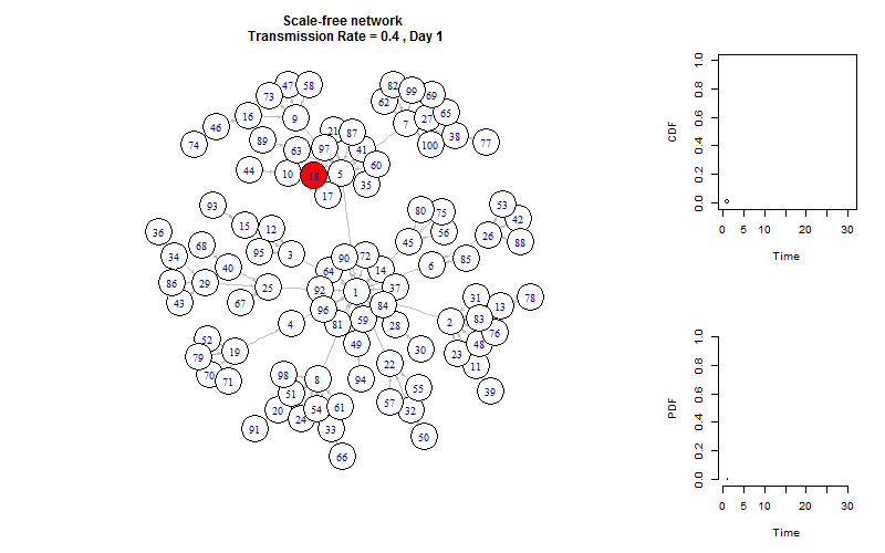
g = barabasi.game(node_number) 
graph_name = "Scale-free network"
plot(g)

plot of chunk unnamed-chunk-7

Initiate the diffusers (Part 1)

seed_num = 1
set.seed(20140301); diffusers = sample(V(g),seed_num)
infected =list()
infected[[1]]= diffusers
# set the color
E(g)$color = "grey"
V(g)$color = "white"

Initiate the diffusers (Part 2)

set.seed(2014); layout.old = layout.fruchterman.reingold(g, niter = 1000)
V(g)$color[V(g)%in%diffusers] = "red"
plot(g, layout =layout.old)

plot of chunk unnamed-chunk-9

Start the contagion!

total_time = 1
while(length(infected[[total_time]]) < node_number){ 
  infected[[total_time+1]] = sort(update_diffusers(infected[[total_time]]))
  cat(length(infected[[total_time+1]]), "-->")
  total_time = total_time + 1
}
2 -->14 -->22 -->29 -->36 -->50 -->59 -->67 -->75 -->80 -->85 -->87 -->88 -->92 -->94 -->97 -->98 -->98 -->98 -->98 -->98 -->99 -->100 -->

Save as the animation (Part 1)

plot_time_series = function(infected, m){
  num_cum = unlist(lapply(1:m, 
            function(x) length(infected[[x]]) ))
  p_cum = num_cum/node_number
  p = diff(c(0, p_cum))
  time = 1:m
  plot(p_cum~time, type = "b", 
       ylab = "CDF", xlab = "Time",
       xlim = c(0,total_time), ylim =c(0,1))
  plot(p~time, type = "h", frame.plot = FALSE,
       ylab = "PDF", xlab = "Time",
       xlim = c(0,total_time), ylim =c(0,1))
}

Save as the animation (Part 1)

plot_time_series(infected, 16)

plot of chunk unnamed-chunk-12 plot of chunk unnamed-chunk-12

Save as the animation (Part 2)

plot_gif = function(infected){
  m = 1
  while(m <= length(infected)){
    layout(matrix(c(1, 2, 1, 3), 2,2, byrow = TRUE), widths=c(3,1), heights=c(1, 1))
    V(g)$color = "white"
    V(g)$color[V(g)%in%infected[[m]]] = "red"
    plot(g, layout =layout.old, edge.arrow.size=0.2)
    title(paste(graph_name, "\n Transmission Rate =", transmission_rate, ", Day", m))
    plot_time_series(infected, m)
    m = m + 1}
}

Save as the animation (Part 3)

library(animation)

saveGIF({
  ani.options(interval = 0.5, convert = shQuote("C:/Program Files/ImageMagick-6.8.8-Q16/convert.exe"))
  # start the plot
  plot_gif(infected)
}, ani.width = 800, ani.height = 500)

See the animation

alt text

This is the end!

Cheng-Jun Wang

  • Web Mining Lab
  • Department of Media and Communication
  • City University of Hong Kong

alt text