
万神殿项目(Pantheon Project)
由塞萨尔·伊达尔戈(César Hidalgo)创建的一个在线工具。
伊达尔戈现在是麻省理工学院媒体实验室的教授,
他曾说:”真正著名的人在他们各自的领域外也相当知名”。
一个人的维基百科页面使用了多少种语言,他就有多大的名气。
若想被列入万神殿,一个人的名气必须跨越国家和语言障碍,必须在维基百科页面上出现至少25种语言。
单单这一个要求就将名人的范围从所有的小名人或不太出名的人缩小到11341人——他们各有特色,魅力十足。
Yu, A. Z., et al. (2016). Pantheon 1.0, a manually verified dataset of globally famous biographies. Scientific Data 2:150075. doi: 10.1038/sdata.2015.75
https://pantheon.world/data/datasets
pantheon.tsv
A tab delimited file containing a row of data per person found in the Panthon 1.0 dataset.
wikilangs.tsv
A tab delimited file of all the different Wikipedia language editions that each biography has a presence in.
pageviews_2008-2013.tsv A file containing the monthly pageview data for each individual, for all the Wikipedia language editions in which they have a presence.
Please refer to the methods section for more information on how this data was created. For detailed descriptions of these datasets, please refer to our data descriptor paper.
Jara-Figueroa, C., Yu, A.Z. and Hidalgo, C.A., 2015. The medium is the memory: how communication technologies shape what we remember. arXiv preprint arXiv:1512.05020.
Yu, A.Z., Ronen, S., Hu, K., Lu, T. and Hidalgo, C.A., 2016. Pantheon 1.0, a manually verified dataset of globally famous biographies. Scientific data, 3.
Ronen, S., Gonçalves, B., Hu, K.Z., Vespignani, A., Pinker, S. and Hidalgo, C.A., 2014. Links that speak: The global language network and its association with global fame. Proceedings of the National Academy of Sciences, 111(52), pp.E5616-E5622.
Cesar A. Hidalgo and Ali Almossawi. “The Data-Visualization Revolution.” Scientific American. March 2014.
Hidalgo, C. A. “The Last 20 Inches: Data’s Treacherous Journey from the Screen to the Mind.” MIT Technology Review. March 2014.
import pandas as pd
import matplotlib.pyplot as plt
import seaborn as sns
df = pd.read_csv('./data/person_2020_update.csv',low_memory=False)
df.head()
| id | wd_id | wp_id | slug | name | occupation | prob_ratio | gender | alive | ... | deathdate | deathyear | bplace_geacron_name | dplace_geacron_name | is_group | l_ | age | non_en_page_views | coefficient_of_variation | hpi | ||
|---|---|---|---|---|---|---|---|---|---|---|---|---|---|---|---|---|---|---|---|---|---|
| 0 | 18934 | Q9458 | 18934 | Muhammad | Muhammad | RELIGIOUS FIGURE | 0.0 | M | NaN | False | ... | 0632-06-08 | 632.0 | Mecca | NaN | False | 27.918400 | 1450.0 | 5160422.0 | 3.199355 | 100.000000 |
| 1 | 17414699 | Q720 | 17414699 | Genghis_Khan | Genghis Khan | MILITARY PERSONNEL | 0.0 | M | NaN | False | ... | 1227-08-18 | 1227.0 | NaN | NaN | False | 25.843621 | 858.0 | 3249211.0 | 2.753641 | 97.723669 |
| 2 | 18079 | Q762 | 18079 | Leonardo_da_Vinci | Leonardo da Vinci | INVENTOR | 0.0 | M | NaN | False | ... | 1519-05-02 | 1519.0 | NaN | NaN | False | 17.545406 | 568.0 | 5362406.0 | 4.796629 | 97.460691 |
| 3 | 14627 | Q935 | 14627 | Isaac_Newton | Isaac Newton | PHYSICIST | 0.0 | M | NaN | False | ... | 1727-03-31 | 1726.0 | NaN | NaN | False | 21.608920 | 378.0 | 3431331.0 | 4.632474 | 96.836567 |
| 4 | 17914 | Q255 | 17914 | Ludwig_van_Beethoven | Ludwig van Beethoven | COMPOSER | 0.0 | M | NaN | False | ... | 1827-03-26 | 1827.0 | NaN | Austria | False | 19.796430 | 250.0 | 5179518.0 | 3.926626 | 96.583969 |
5 rows × 34 columns
len(df)
88937
df.iloc[0]
id 18934
wd_id Q9458
wp_id 18934
slug Muhammad
name Muhammad
occupation RELIGIOUS FIGURE
prob_ratio 0.000000
gender M
twitter NaN
alive False
l 193
hpi_raw 36
bplace_name Mecca
bplace_lat 21.416667
bplace_lon 39.816667
bplace_geonameid 21021.000000
bplace_country Saudi Arabia
birthdate NaN
birthyear 570.000000
dplace_name Medina
dplace_lat 24.466667
dplace_lon 39.600000
dplace_geonameid 36636.000000
dplace_country Saudi Arabia
deathdate 0632-06-08
deathyear 632.000000
bplace_geacron_name Mecca
dplace_geacron_name NaN
is_group False
l_ 27.918400
age 1450.000000
non_en_page_views 5160422.000000
coefficient_of_variation 3.199355
hpi 100.000000
age_group (1003.333, 2006.667]
Name: 0, dtype: object
df.columns
Index(['id', 'wd_id', 'wp_id', 'slug', 'name', 'occupation', 'prob_ratio',
'gender', 'twitter', 'alive', 'l', 'hpi_raw', 'bplace_name',
'bplace_lat', 'bplace_lon', 'bplace_geonameid', 'bplace_country',
'birthdate', 'birthyear', 'dplace_name', 'dplace_lat', 'dplace_lon',
'dplace_geonameid', 'dplace_country', 'deathdate', 'deathyear',
'bplace_geacron_name', 'dplace_geacron_name', 'is_group', 'l_', 'age',
'non_en_page_views', 'coefficient_of_variation', 'hpi'],
dtype='object')
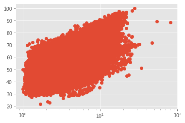
The HPI combines the number of languages L, the effective number of languages L*, the age of the historical character A, the number of PageViews in Non-English Wikipedias v_NE (calculated in 2016), and the coefficient of variation in PageViews in all languages between CV (also calculated in 2016).
https://pantheon.world/about/methods
plt.style.use('ggplot')
plt.plot(df['l_'], df['hpi'], 'o')
plt.xscale('log')
plt.show()
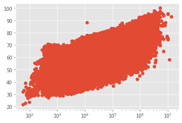
plt.style.use('ggplot')
plt.plot(df['non_en_page_views'], df['hpi'], 'o')
plt.xscale('log')
plt.show()
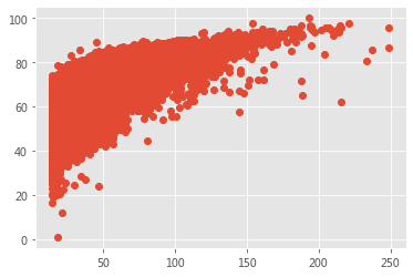
plt.style.use('ggplot')
plt.plot(df['l'], df['hpi'], 'o')
#plt.xscale('log')
plt.show()
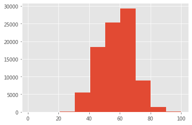
plt.hist(df['hpi']);
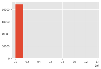
plt.hist(df['non_en_page_views']);
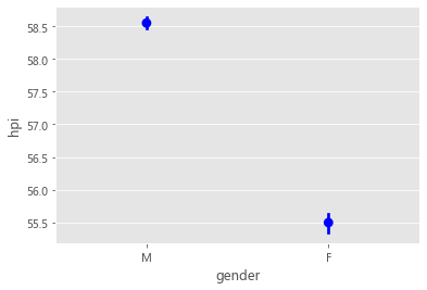
sns.pointplot(x='gender', y = 'hpi', data = df, color = 'blue', linestyles='');
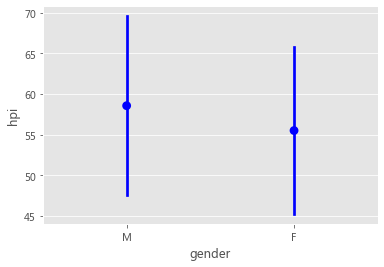
sns.pointplot(x='gender', y = 'hpi', ci = 'sd', data = df, color = 'blue', linestyles='');
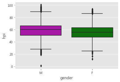
sns.boxplot(x="gender", y="hpi",
#hue="smoker",
palette=["m", "g"],
data=df);
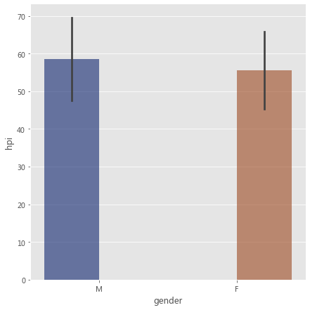
# Draw a nested barplot by species and sex
g = sns.catplot(
data=df, kind="bar",
x="gender", y="hpi", hue="gender",
ci="sd", palette="dark", alpha=.6, height=6
)
df['age_group']=pd.cut(df['age'], bins = 6)
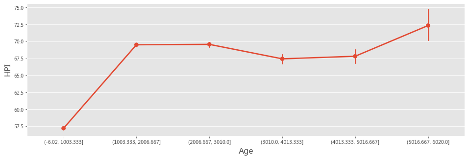
plt.figure(figsize = (16, 5))
sns.pointplot(x="age_group", y="hpi", data=df)
plt.xlabel('Age', fontsize = 16)
plt.ylabel('HPI', fontsize = 16)
plt.show()
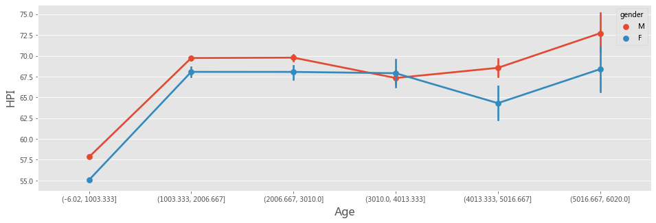
plt.figure(figsize = (16, 5))
sns.pointplot(x="age_group", y="hpi", data=df, hue = 'gender')
plt.xlabel('Age', fontsize = 16)
plt.ylabel('HPI', fontsize = 16)
plt.show()
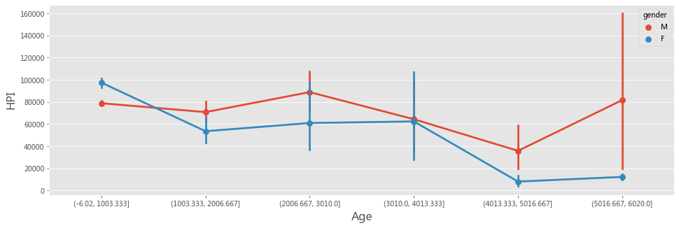
plt.figure(figsize = (16, 5))
sns.pointplot(x="age_group", y="non_en_page_views", data=df, hue = 'gender')
plt.xlabel('Age', fontsize = 16)
plt.ylabel('HPI', fontsize = 16)
plt.show()
plt.figure(figsize = (16, 5))
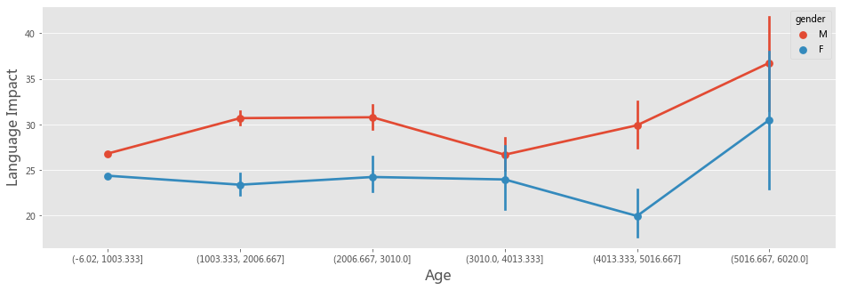
sns.pointplot(x="age_group", y="l", data=df, hue = 'gender')
plt.xlabel('Age', fontsize = 16)
plt.ylabel('Language Impact', fontsize = 16)
plt.show()
plt.figure(figsize = (16, 5))
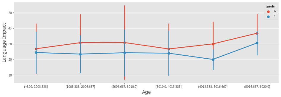
sns.pointplot(x="age_group", y="l", ci = 'sd', data=df, hue = 'gender')
plt.xlabel('Age', fontsize = 16)
plt.ylabel('Language Impact', fontsize = 16)
plt.show()
df['occupation'].unique()
array(['RELIGIOUS FIGURE', 'MILITARY PERSONNEL', 'INVENTOR', 'PHYSICIST',
'COMPOSER', 'PHILOSOPHER', 'POLITICIAN', 'ASTRONOMER', 'EXPLORER',
'PAINTER', 'WRITER', 'MATHEMATICIAN', 'PSYCHOLOGIST',
'SOCIAL ACTIVIST', 'BIOLOGIST', 'ECONOMIST', 'NOBLEMAN', 'BOXER',
'HISTORIAN', 'ACTOR', 'CHEMIST', 'PHYSICIAN', 'SOCIOLOGIST',
'SOCCER PLAYER', 'OCCULTIST', 'ASTRONAUT', 'COMPANION', 'DESIGNER',
'MUSICIAN', 'SINGER', 'ARCHITECT', 'INSPIRATION', 'EXTREMIST',
'FILM DIRECTOR', 'COMPUTER SCIENTIST', 'DIPLOMAT', 'PRODUCER',
'GEOGRAPHER', 'MAFIOSO', 'PILOT', 'BUSINESSPERSON',
'FASHION DESIGNER', 'ARTIST', 'CELEBRITY', 'SCULPTOR', 'ENGINEER',
'DANCER', 'PIRATE', 'LINGUIST', 'LAWYER', 'COMEDIAN',
'ARCHAEOLOGIST', 'MARTIAL ARTS', 'COMIC ARTIST', 'ATHLETE',
'COACH', 'RACING DRIVER', 'MAGICIAN', 'GEOLOGIST', 'CONDUCTOR',
'MOUNTAINEER', 'PUBLIC WORKER', 'CHESS PLAYER', 'JUDGE',
'JOURNALIST', 'POLITICAL SCIENTIST', 'ANTHROPOLOGIST',
'PHOTOGRAPHER', 'SWIMMER', 'PORNOGRAPHIC ACTOR', 'CYCLIST',
'TENNIS PLAYER', 'AMERICAN FOOTBALL PLAYER', 'STATISTICIAN',
'BASKETBALL PLAYER', 'PRESENTER', 'MODEL', 'CRITIC', 'SKATER',
'BASEBALL PLAYER', 'GYMNAST', 'WRESTLER', 'REFEREE', 'BULLFIGHTER',
'GAME DESIGNER', 'YOUTUBER', 'SKIER', 'CHEF', 'GO PLAYER',
'HOCKEY PLAYER', 'FENCER', 'GOLFER', 'POKER PLAYER',
'TABLE TENNIS PLAYER', 'SNOOKER', 'CRICKETER', 'HANDBALL PLAYER',
'VOLLEYBALL PLAYER', 'RUGBY PLAYER', 'GAMER', 'BADMINTON PLAYER'],
dtype=object)
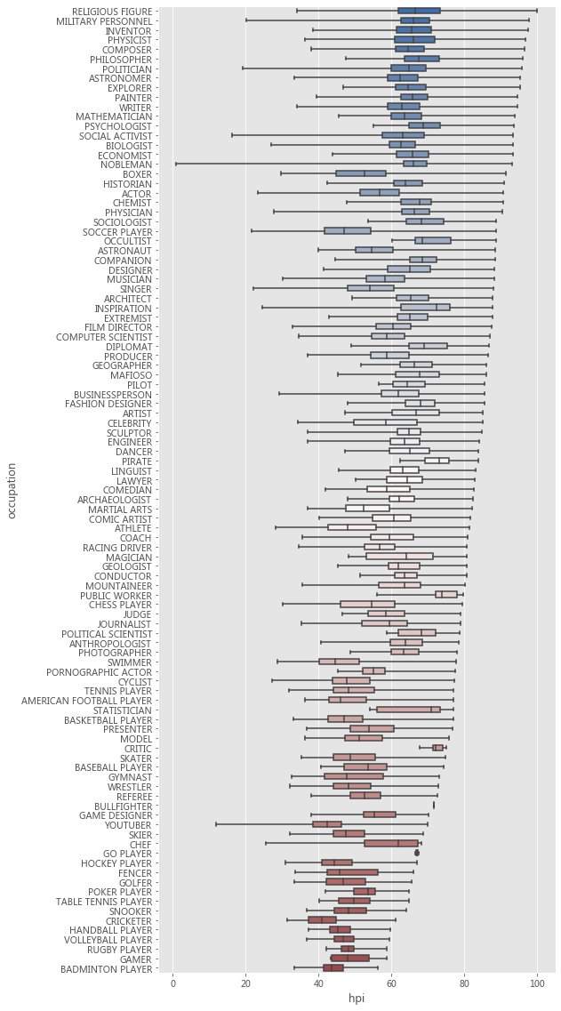
plt.figure(figsize = (8, 20))
sns.boxplot(x="hpi", y="occupation", data=df,
whis=[0, 100], width=.6, palette="vlag");
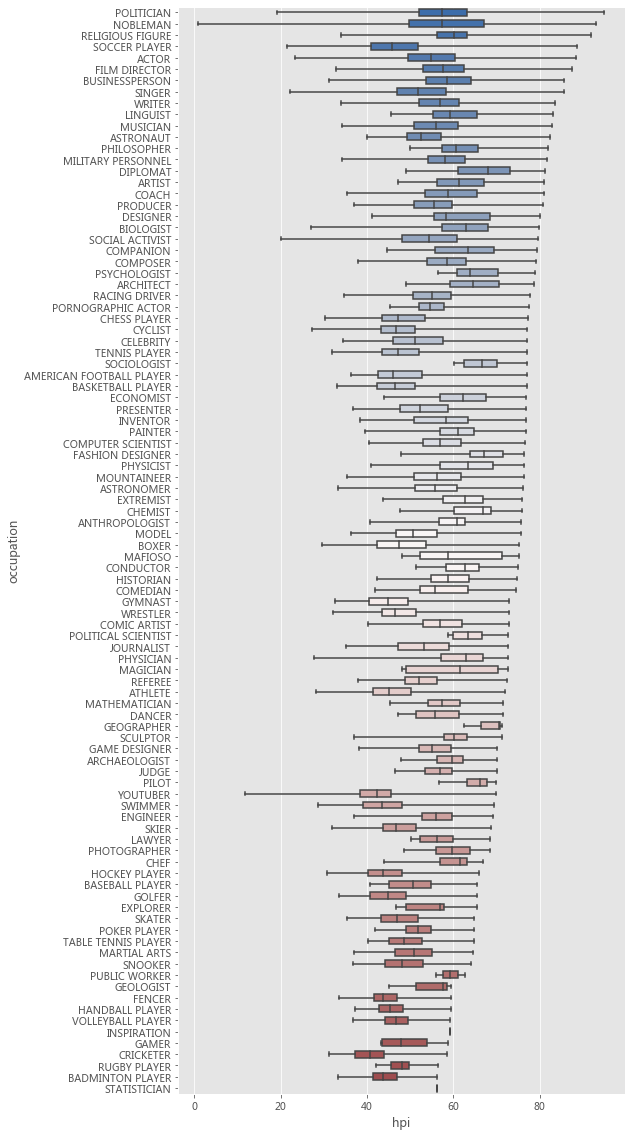
plt.figure(figsize = (8, 20))
sns.boxplot(x="hpi", y="occupation", data=df[df['alive']==True],
whis=[0, 100], width=.6, palette="vlag");
import numpy as np
dat = df[(pd.isna(df['bplace_lat'])==False) &(pd.isna(df['dplace_lat'])==False)]
len(dat)
36123
dat0 = dat[dat['birthyear']<=0]
len(dat0)
700
dat0['name']
5 Alexander the Great
6 Aristotle
8 Julius Caesar
10 Plato
11 Jesus
...
42995 Prince Vijaya
43349 Seleucus VII Philometor
45324 Panyassis
46802 Alexis
54763 Agathokleia
Name: name, Length: 700, dtype: object
import plotly.graph_objects as go
fig = go.Figure()
#'bplace_lat', 'bplace_lon','dplace_lat', 'dplace_lon'
fig.add_trace(go.Scattergeo(
#locationmode = 'USA-states',
lon = dat0['bplace_lon'],
lat = dat0['bplace_lat'],
hovertext = dat0['name'],
mode = 'markers',
marker = dict(
size = 2,
color = 'rgb(255, 0, 0)',
line = dict(
width = 3,
color = 'rgba(68, 68, 68, 0)'
)
)))
fig.update_layout(
title_text = 'Pantheon Project',
showlegend = False,
geo = dict(
scope = 'world',
projection_type = 'natural earth',
showland = True,
landcolor = 'rgb(243, 243, 243)',
countrycolor = 'rgb(204, 204, 204)',
),
)
fig.show()
import plotly.graph_objects as go
fig = go.Figure()
#'bplace_lat', 'bplace_lon','dplace_lat', 'dplace_lon'
for i in dat0.index:
fig.add_trace(
go.Scattergeo(
#locationmode = 'USA-states',
lon = [dat0['bplace_lon'][i], dat0['dplace_lon'][i]],
lat = [dat0['bplace_lat'][i], dat0['dplace_lat'][i]],
mode = 'lines',
line = dict(width = 1,color = 'red'),
opacity = 0.5,
hovertext = dat0['name'],
hoverinfo="text",
)
)
fig.update_layout(
title_text = 'Pantheon Project',
showlegend = False,
geo = dict(
scope = 'world',
projection_type = 'natural earth',
showland = True,
landcolor = 'rgb(243, 243, 243)',
countrycolor = 'rgb(204, 204, 204)',
),
)
fig.show()