Causal Forests#
install.packages('grf')
The downloaded binary packages are in
	/var/folders/8b/hhnbt0nd4zsg2qhxc28q23w80000gn/T//RtmpydKe1A/downloaded_packages
library('grf')
Warning message:
“package ‘grf’ was built under R version 3.6.2”
if(packageVersion("grf") < '0.10.2') {
  warning("This script requires grf 0.10.2 or higher")
}
library(sandwich)
library(lmtest)
library(Hmisc)
library(ggplot2)
set.seed(1)

rm(list = ls())
data.all = read.csv("./data/synthetic_data.csv")
data.all$schoolid = factor(data.all$schoolid)

DF = data.all[,-1]
school.id = as.numeric(data.all$schoolid)

school.mat = model.matrix(~ schoolid + 0, data = data.all)
school.size = colSums(school.mat)
# It appears that school ID does not affect pscore. So ignore it
# in modeling, and just treat it as source of per-cluster error.
w.lm = glm(Z ~ ., data = data.all[,-3], family = binomial)
summary(w.lm)
Call:
glm(formula = Z ~ ., family = binomial, data = data.all[, -3])

Deviance Residuals:
    Min       1Q   Median       3Q      Max
-1.2079  -0.9088  -0.8297   1.4176   1.9556

Coefficients: (6 not defined because of singularities)
              Estimate Std. Error z value Pr(>|z|)
(Intercept) -0.9524636  0.2845173  -3.348 0.000815 ***
schoolid2    0.0697302  0.2766287   0.252 0.800986
schoolid3    0.0382080  0.2911323   0.131 0.895586
schoolid4    0.1761334  0.2784711   0.633 0.527059
schoolid5   -0.0033389  0.2950180  -0.011 0.990970
schoolid6    0.0583548  0.3067481   0.190 0.849124
schoolid7   -0.1313759  0.3188190  -0.412 0.680288
schoolid8    0.1233661  0.3023736   0.408 0.683279
schoolid9   -0.1955428  0.3073344  -0.636 0.524611
schoolid10  -0.1892794  0.2968750  -0.638 0.523752
schoolid11  -0.2224060  0.5461005  -0.407 0.683816
schoolid12  -0.3312420  0.5414374  -0.612 0.540682
schoolid13  -0.0408540  0.3989507  -0.102 0.918436
schoolid14  -0.8681934  0.6033674  -1.439 0.150175
schoolid15  -0.1059135  0.3263162  -0.325 0.745504
schoolid16  -0.1063268  0.2885387  -0.369 0.712500
schoolid17   0.0854323  0.3119435   0.274 0.784184
schoolid18  -0.1924441  0.2997822  -0.642 0.520908
schoolid19  -0.0265326  0.3229712  -0.082 0.934526
schoolid20  -0.2179554  0.3041336  -0.717 0.473594
schoolid21  -0.2147440  0.2982822  -0.720 0.471565
schoolid22  -0.5115966  0.4410779  -1.160 0.246098
schoolid23   0.0039231  0.3475373   0.011 0.990994
schoolid24  -0.0848314  0.3259572  -0.260 0.794668
schoolid25   0.0521087  0.2754586   0.189 0.849959
schoolid26   0.0241212  0.2876511   0.084 0.933171
schoolid27  -0.2300630  0.3104796  -0.741 0.458698
schoolid28  -0.3519010  0.2924774  -1.203 0.228909
schoolid29  -0.2198764  0.3293288  -0.668 0.504357
schoolid30  -0.3146292  0.3257994  -0.966 0.334187
schoolid31   0.1398555  0.6137901   0.228 0.819759
schoolid32   0.1555524  0.3916156   0.397 0.691215
schoolid33  -0.0991693  0.3939370  -0.252 0.801243
schoolid34  -0.0073688  0.2980808  -0.025 0.980278
schoolid35  -0.3528987  0.3997273  -0.883 0.377318
schoolid36  -0.3751465  0.3988972  -0.940 0.346982
schoolid37  -0.0343169  0.3219646  -0.107 0.915117
schoolid38  -0.1346432  0.3851869  -0.350 0.726674
schoolid39  -0.4339936  0.3612869  -1.201 0.229657
schoolid40  -0.3993958  0.3834495  -1.042 0.297604
schoolid41  -0.1490784  0.3542105  -0.421 0.673846
schoolid42  -0.1545715  0.3551857  -0.435 0.663428
schoolid43  -0.5679567  0.4277455  -1.328 0.184247
schoolid44  -0.1425896  0.3774795  -0.378 0.705623
schoolid45  -0.1337888  0.3232493  -0.414 0.678957
schoolid46  -0.2573249  0.3129119  -0.822 0.410874
schoolid47   0.0027726  0.2770108   0.010 0.992014
schoolid48  -0.3406079  0.3470361  -0.981 0.326358
schoolid49  -0.3236117  0.3434541  -0.942 0.346077
schoolid50  -0.1185119  0.4086074  -0.290 0.771787
schoolid51   0.4087898  0.4506822   0.907 0.364382
schoolid52  -0.3144014  0.4118342  -0.763 0.445214
schoolid53  -0.2733677  0.4511280  -0.606 0.544538
schoolid54  -0.0889588  0.3872532  -0.230 0.818311
schoolid55  -0.1558106  0.4155020  -0.375 0.707665
schoolid56   0.1050353  0.3149235   0.334 0.738737
schoolid57  -0.0314901  0.2901719  -0.109 0.913581
schoolid58  -0.0383183  0.2730077  -0.140 0.888379
schoolid59  -0.0529637  0.2934895  -0.180 0.856790
schoolid60  -0.1624792  0.3972885  -0.409 0.682561
schoolid61  -0.0289549  0.3201953  -0.090 0.927946
schoolid62   0.0993158  0.2669678   0.372 0.709882
schoolid63   0.1684702  0.3282167   0.513 0.607749
schoolid64  -0.0693060  0.2770896  -0.250 0.802493
schoolid65  -0.0004197  0.4072922  -0.001 0.999178
schoolid66  -0.2130911  0.2984091  -0.714 0.475171
schoolid67   0.0358440  0.2921158   0.123 0.902341
schoolid68  -0.0871303  0.3290814  -0.265 0.791188
schoolid69  -0.2550387  0.2908992  -0.877 0.380636
schoolid70  -0.0268947  0.4032160  -0.067 0.946820
schoolid71   0.0037464  0.4268290   0.009 0.992997
schoolid72  -0.1304085  0.2881512  -0.453 0.650859
schoolid73  -0.2160697  0.2840030  -0.761 0.446776
schoolid74  -0.0935320  0.2842612  -0.329 0.742129
schoolid75  -0.1056241  0.3024204  -0.349 0.726892
schoolid76  -0.1052261  0.2939262  -0.358 0.720342
S3           0.1036077  0.0197345   5.250 1.52e-07 ***
C1          -0.0015919  0.0053900  -0.295 0.767728
C2          -0.1038596  0.0424020  -2.449 0.014309 *
C3          -0.1319218  0.0461833  -2.856 0.004284 **
XC                  NA         NA      NA       NA
X1                  NA         NA      NA       NA
X2                  NA         NA      NA       NA
X3                  NA         NA      NA       NA
X4                  NA         NA      NA       NA
X5                  NA         NA      NA       NA
---
Signif. codes:  0 ‘***’ 0.001 ‘**’ 0.01 ‘*’ 0.05 ‘.’ 0.1 ‘ ’ 1

(Dispersion parameter for binomial family taken to be 1)

    Null deviance: 13115  on 10390  degrees of freedom
Residual deviance: 13009  on 10311  degrees of freedom
AIC: 13169

Number of Fisher Scoring iterations: 4
W = DF$Z
Y = DF$Y
X.raw = DF[,-(1:2)]

C1.exp = model.matrix(~ factor(X.raw$C1) + 0)
XC.exp = model.matrix(~ factor(X.raw$XC) + 0)

X = cbind(X.raw[,-which(names(X.raw) %in% c("C1", "XC"))], C1.exp, XC.exp)
#
# Grow a forest. Add extra trees for the causal forest.
#

Y.forest = regression_forest(X, Y, clusters = school.id, equalize.cluster.weights = TRUE)
Y.hat = predict(Y.forest)$predictions
W.forest = regression_forest(X, W, clusters = school.id, equalize.cluster.weights = TRUE)
W.hat = predict(W.forest)$predictions

cf.raw = causal_forest(X, Y, W,
                       Y.hat = Y.hat, W.hat = W.hat,
                       clusters = school.id,
                       equalize.cluster.weights = TRUE)
varimp = variable_importance(cf.raw)
selected.idx = which(varimp > mean(varimp))

cf = causal_forest(X[,selected.idx], Y, W,
                   Y.hat = Y.hat, W.hat = W.hat,
                   clusters = school.id,
                   equalize.cluster.weights = TRUE,
                   tune.parameters = "all")
tau.hat = predict(cf)$predictions
#
# Estimate ATE
#

ATE = average_treatment_effect(cf)
paste("95% CI for the ATE:", round(ATE[1], 3),
      "+/-", round(qnorm(0.975) * ATE[2], 3))
'95% CI for the ATE: 0.249 +/- 0.04'
#
# Omnibus tests for heterogeneity
#

# Run best linear predictor analysis
test_calibration(cf)

# Compare regions with high and low estimated CATEs
high_effect = tau.hat > median(tau.hat)
ate.high = average_treatment_effect(cf, subset = high_effect)
ate.low = average_treatment_effect(cf, subset = !high_effect)
paste("95% CI for difference in ATE:",
      round(ate.high[1] - ate.low[1], 3), "+/-",
      round(qnorm(0.975) * sqrt(ate.high[2]^2 + ate.low[2]^2), 3))
Best linear fit using forest predictions (on held-out data)
as well as the mean forest prediction as regressors, along
with one-sided heteroskedasticity-robust (HC3) SEs:

                                Estimate Std. Error t value Pr(>t)
mean.forest.prediction          1.008054   0.082129 12.2741 <2e-16 ***
differential.forest.prediction -0.552783   1.063927 -0.5196 0.6983
---
Signif. codes:  0 ‘***’ 0.001 ‘**’ 0.01 ‘*’ 0.05 ‘.’ 0.1 ‘ ’ 1
'95% CI for difference in ATE: 0.01 +/- 0.074'
#
# formal test for X1 and X2
#

dr.score = tau.hat + W / cf$W.hat *
  (Y - cf$Y.hat - (1 - cf$W.hat) * tau.hat) -
  (1 - W) / (1 - cf$W.hat) * (Y - cf$Y.hat + cf$W.hat * tau.hat)
school.score = t(school.mat) %*% dr.score / school.size

school.X1 = t(school.mat) %*% X$X1 / school.size
high.X1 = school.X1 > median(school.X1)
t.test(school.score[high.X1], school.score[!high.X1])

school.X2 = (t(school.mat) %*% X$X2) / school.size
high.X2 = school.X2 > median(school.X2)
t.test(school.score[high.X2], school.score[!high.X2])

school.X2.levels = cut(school.X2,
  breaks = c(-Inf, quantile(school.X2, c(1/3, 2/3)), Inf))
summary(aov(school.score ~ school.X2.levels))
	Welch Two Sample t-test

data:  school.score[high.X1] and school.score[!high.X1]
t = -3.0347, df = 71.45, p-value = 0.003357
alternative hypothesis: true difference in means is not equal to 0
95 percent confidence interval:
 -0.19218352 -0.03978437
sample estimates:
mean of x mean of y
0.1908525 0.3068365
	Welch Two Sample t-test

data:  school.score[high.X2] and school.score[!high.X2]
t = 0.9637, df = 72.286, p-value = 0.3384
alternative hypothesis: true difference in means is not equal to 0
95 percent confidence interval:
 -0.04146936  0.11909811
sample estimates:
mean of x mean of y
0.2682517 0.2294373
                 Df Sum Sq Mean Sq F value Pr(>F)
school.X2.levels  2 0.0811 0.04054   1.328  0.271
Residuals        73 2.2283 0.03052
#
# formal test for S3
#

school.score.XS3.high = t(school.mat) %*% (dr.score * (X$S3 >= 6)) /
  t(school.mat) %*% (X$S3 >= 6)
school.score.XS3.low = t(school.mat) %*% (dr.score * (X$S3 < 6)) /
  t(school.mat) %*% (X$S3 < 6)

plot(school.score.XS3.low, school.score.XS3.high)
t.test(school.score.XS3.high - school.score.XS3.low)
	One Sample t-test

data:  school.score.XS3.high - school.score.XS3.low
t = 2.2397, df = 75, p-value = 0.02807
alternative hypothesis: true mean is not equal to 0
95 percent confidence interval:
 0.009408619 0.160803922
sample estimates:
 mean of x
0.08510627

#
# Look at school-wise heterogeneity
#

#pdf("school_hist.pdf")
pardef = par(mar = c(5, 4, 4, 2) + 0.5, cex.lab=1.5, cex.axis=1.5, cex.main=1.5, cex.sub=1.5)
hist(school.score, xlab = "School Treatment Effect Estimate", main = "")
#dev.off()

#
# Re-check ATE... sanity check only
#

ate.hat = mean(school.score)
se.hat = sqrt(var(school.score) / length(school.score - 1))
print(paste(round(ate.hat, 3), "+/-", round(1.96 * se.hat, 3)))
[1] "0.249 +/- 0.039"
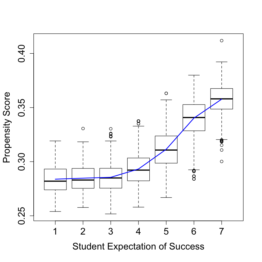
#
# Look at variation in propensity scores
#

DF = X
DF$W.hat = cf$W.hat

#pdf("pscore.pdf")
pardef = par(mar = c(5, 4, 4, 2) + 0.5, cex.lab=1.5, cex.axis=1.5, cex.main=1.5, cex.sub=1.5)
boxplot(W.hat ~ S3, data = DF, ylab = "Propensity Score", xlab = "Student Expectation of Success")
lines(smooth.spline(X$S3, cf$W.hat), lwd = 2, col = 4)
#dev.off()
#
# Analysis ignoring clusters
#

cf.noclust = causal_forest(X[,selected.idx], Y, W,
                           Y.hat = Y.hat, W.hat = W.hat,
                           tune.parameters = "all")

ATE.noclust = average_treatment_effect(cf.noclust)
paste("95% CI for the ATE:", round(ATE.noclust[1], 3),
      "+/-", round(qnorm(0.975) * ATE.noclust[2], 3))

test_calibration(cf.noclust)

tau.hat.noclust = predict(cf.noclust)$predict
plot(school.id, tau.hat.noclust)

nfold = 5
school.levels = unique(school.id)
cluster.folds = sample.int(nfold, length(school.levels), replace = TRUE)

tau.hat.crossfold = rep(NA, length(Y))
for (foldid in 1:nfold) {
  print(foldid)
  infold = school.id %in% school.levels[cluster.folds == foldid]
  cf.fold = causal_forest(X[!infold, selected.idx], Y[!infold], W[!infold],
                          Y.hat = Y.hat[!infold], W.hat = W.hat[!infold],
                          tune.parameters = "all")
  pred.fold = predict(cf.fold, X[infold, selected.idx])$predictions
  tau.hat.crossfold[infold] = pred.fold
}

cf.noclust.cpy = cf.noclust
cf.noclust.cpy$predictions = tau.hat.crossfold
cf.noclust.cpy$clusters = school.id
test_calibration(cf.noclust.cpy)

Rloss = mean(((Y - Y.hat) - tau.hat * (W - W.hat))^2)
Rloss.noclust = mean(((Y - Y.hat) - tau.hat.noclust * (W - W.hat))^2)
Rloss.crossfold = mean(((Y - Y.hat) - tau.hat.crossfold * (W - W.hat))^2)

c(Rloss.noclust - Rloss, Rloss.crossfold - Rloss)

summary(aov(dr.score ~ factor(school.id)))
'95% CI for the ATE: 0.254 +/- 0.022'
Best linear fit using forest predictions (on held-out data)
as well as the mean forest prediction as regressors, along
with one-sided heteroskedasticity-robust (HC3) SEs:

                               Estimate Std. Error t value    Pr(>t)
mean.forest.prediction         1.012757   0.045084 22.4639 < 2.2e-16 ***
differential.forest.prediction 0.528275   0.133245  3.9647 3.699e-05 ***
---
Signif. codes:  0 ‘***’ 0.001 ‘**’ 0.01 ‘*’ 0.05 ‘.’ 0.1 ‘ ’ 1
[1] 1
[1] 2
[1] 3
[1] 4
[1] 5
Best linear fit using forest predictions (on held-out data)
as well as the mean forest prediction as regressors, along
with one-sided heteroskedasticity-robust (HC3) SEs:

                               Estimate Std. Error t value Pr(>t)
mean.forest.prediction         0.988134   0.064817 15.2450 <2e-16 ***
differential.forest.prediction 0.224634   0.213643  1.0514 0.1465
---
Signif. codes:  0 ‘***’ 0.001 ‘**’ 0.01 ‘*’ 0.05 ‘.’ 0.1 ‘ ’ 1
- -8.91498516542577e-05
- 0.000504054002137821
                     Df Sum Sq Mean Sq F value   Pr(>F)
factor(school.id)    75    201   2.677    1.98 1.05e-06 ***
Residuals         10315  13944   1.352
---
Signif. codes:  0 ‘***’ 0.001 ‘**’ 0.01 ‘*’ 0.05 ‘.’ 0.1 ‘ ’ 1

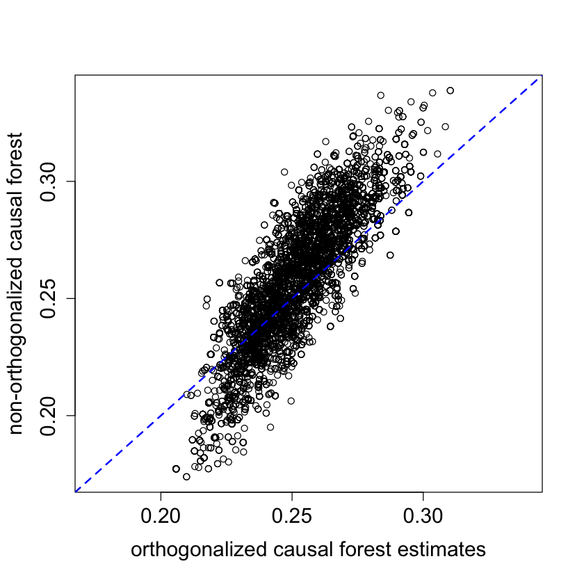
#
# Analaysis without fitting the propensity score
#

cf.noprop = causal_forest(X[,selected.idx], Y, W,
                          Y.hat = Y.hat, W.hat = mean(W),
                          tune.parameters = "all",
                          equalize.cluster.weights = TRUE,
                          clusters = school.id)
tau.hat.noprop = predict(cf.noprop)$predictions

ATE.noprop = average_treatment_effect(cf.noprop)
paste("95% CI for the ATE:", round(ATE.noprop[1], 3),
      "+/-", round(qnorm(0.975) * ATE.noprop[2], 3))

#pdf("tauhat_noprop.pdf")
pardef = par(mar = c(5, 4, 4, 2) + 0.5, cex.lab=1.5, cex.axis=1.5, cex.main=1.5, cex.sub=1.5)
plot(tau.hat, tau.hat.noprop,
     xlim = range(tau.hat, tau.hat.noprop),
     ylim = range(tau.hat, tau.hat.noprop),
     xlab = "orthogonalized causal forest estimates",
     ylab = "non-orthogonalized causal forest")
abline(0, 1, lwd = 2, lty = 2, col = 4)
par = pardef
#dev.off()
'95% CI for the ATE: 0.255 +/- 0.041'
#
# Train forest on school-wise DR scores
#

school.X = (t(school.mat) %*% as.matrix(X[,c(4:8, 25:28)])) / school.size
school.X = data.frame(school.X)
colnames(school.X) = c("X1", "X2", "X3", "X4", "X5",
                    "XC.1", "XC.2", "XC.3", "XC.4")

dr.score = tau.hat + W / cf$W.hat * (Y - cf$Y.hat - (1 - cf$W.hat) * tau.hat) -
  (1 - W) / (1 - cf$W.hat) * (Y - cf$Y.hat + cf$W.hat * tau.hat)
school.score = t(school.mat) %*% dr.score / school.size

school.forest = regression_forest(school.X, school.score)
school.pred = predict(school.forest)$predictions
test_calibration(school.forest)


# Alternative OLS analysis
school.DF = data.frame(school.X, school.score=school.score)
coeftest(lm(school.score ~ ., data = school.DF), vcov = vcovHC)
Best linear fit using forest predictions (on held-out data)
as well as the mean forest prediction as regressors, along
with one-sided heteroskedasticity-robust (HC3) SEs:

                               Estimate Std. Error t value Pr(>t)
mean.forest.prediction          1.00004    0.08179 12.2269 <2e-16 ***
differential.forest.prediction  0.71717    0.67983  1.0549 0.1474
---
Signif. codes:  0 ‘***’ 0.001 ‘**’ 0.01 ‘*’ 0.05 ‘.’ 0.1 ‘ ’ 1
t test of coefficients:

              Estimate Std. Error t value Pr(>|t|)
(Intercept)  0.2414116  0.0770612  3.1327 0.002583 **
X1          -0.0506340  0.0291568 -1.7366 0.087121 .
X2           0.0125656  0.0336563  0.3734 0.710084
X3           0.0102119  0.0266019  0.3839 0.702302
X4           0.0236645  0.0255092  0.9277 0.356950
X5          -0.0357828  0.0268560 -1.3324 0.187312
XC.1         0.0015231  0.0935067  0.0163 0.987054
XC.2         0.0887259  0.1047433  0.8471 0.400012
XC.3        -0.1341513  0.0875327 -1.5326 0.130158
XC.4         0.0424028  0.0816170  0.5195 0.605127
---
Signif. codes:  0 ‘***’ 0.001 ‘**’ 0.01 ‘*’ 0.05 ‘.’ 0.1 ‘ ’ 1
#
# Make some plots...
#

#pdf("tauhat_hist.pdf")
pardef = par(mar = c(5, 4, 4, 2) + 0.5, cex.lab=1.5, cex.axis=1.5, cex.main=1.5, cex.sub=1.5)
hist(tau.hat, xlab = "estimated CATE", main = "")
#dev.off()

#pdf("tauhat_hist_noprop.pdf")
pardef = par(mar = c(5, 4, 4, 2) + 0.5, cex.lab=1.5, cex.axis=1.5, cex.main=1.5, cex.sub=1.5)
hist(tau.hat.noprop, xlab = "estimated CATE", main = "")
#dev.off()

#pdf("tauhat_hist_noclust.pdf")
pardef = par(mar = c(5, 4, 4, 2) + 0.5, cex.lab=1.5, cex.axis=1.5, cex.main=1.5, cex.sub=1.5)
hist(tau.hat.noclust, xlab = "estimated CATE", main = "",
     breaks = seq(-0.0, 0.55, by = 0.55 / 25))
#dev.off()

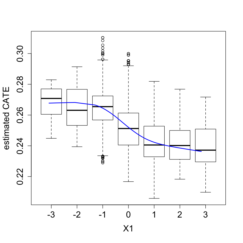
#pdf("tauhat_vs_X1.pdf")
pardef = par(mar = c(5, 4, 4, 2) + 0.5, cex.lab=1.5, cex.axis=1.5, cex.main=1.5, cex.sub=1.5)
boxplot(tau.hat ~ round(X$X1), xlab = "X1", ylab = "estimated CATE")
lines(smooth.spline(4 + X[,"X1"], tau.hat, df = 4), lwd = 2, col = 4)
#dev.off()
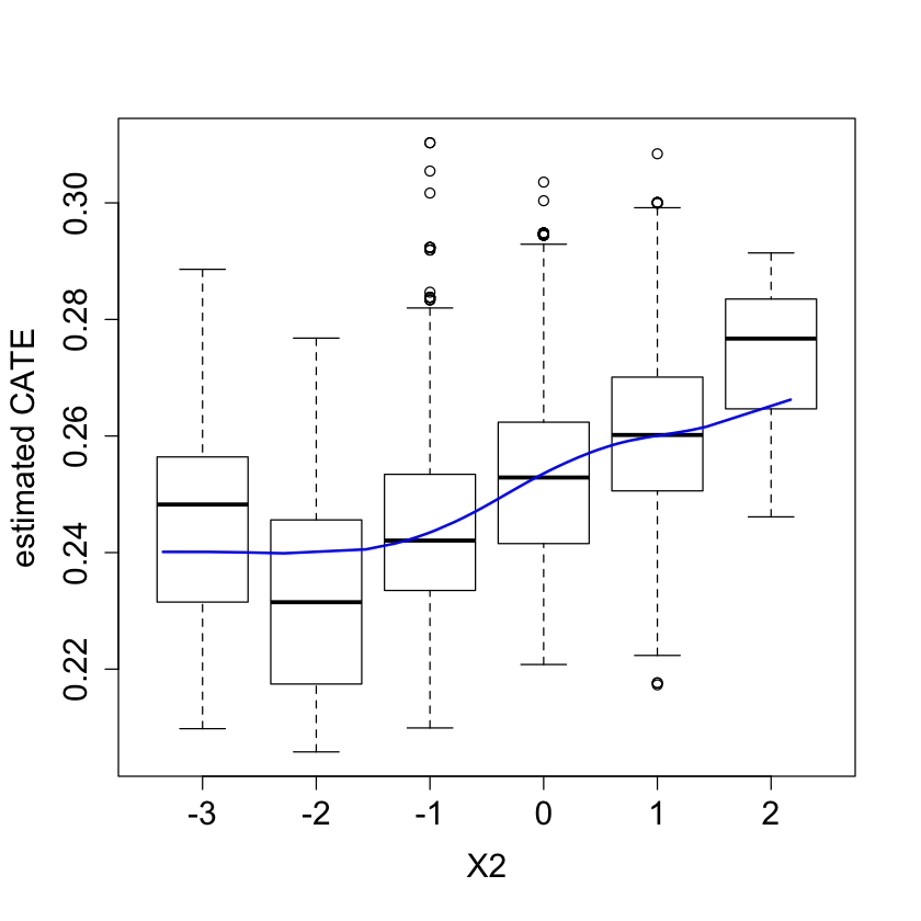
#pdf("tauhat_vs_X2.pdf")
pardef = par(mar = c(5, 4, 4, 2) + 0.5, cex.lab=1.5, cex.axis=1.5, cex.main=1.5, cex.sub=1.5)
boxplot(tau.hat ~ round(X$X2), xlab = "X2", ylab = "estimated CATE")
lines(smooth.spline(4 + X[,"X2"], tau.hat, df = 4), lwd = 2, col = 4)
#dev.off()
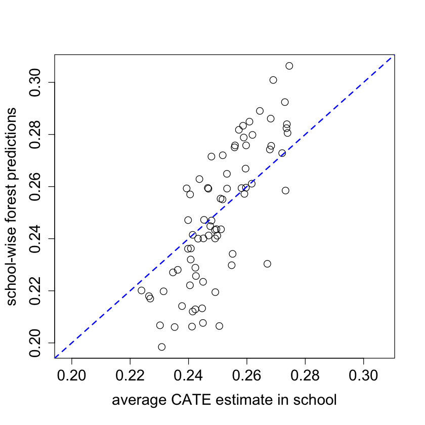
school.avg.tauhat = t(school.mat) %*% tau.hat / school.size

#pdf("school_avg.pdf")
pardef = par(mar = c(5, 4, 4, 2) + 0.5, cex.lab=1.5, cex.axis=1.5, cex.main=1.5, cex.sub=1.5)
plot(school.avg.tauhat, school.pred, cex = 1.5,
     xlim = range(school.avg.tauhat, school.pred),
     ylim = range(school.avg.tauhat, school.pred),
     xlab = "average CATE estimate in school",
     ylab = "school-wise forest predictions")
abline(0, 1, lwd = 2, lty = 2, col = 4)
par = pardef
#dev.off()
#
# Experiment with no orthogonalization
#

n.synth = 1000
p.synth = 10
X.synth = matrix(rnorm(n.synth * p.synth), n.synth, p.synth)
W.synth = rbinom(n.synth, 1, 1 / (1 + exp(-X.synth[,1])))
Y.synth = 2 * rowMeans(X.synth[,1:6]) + rnorm(n.synth)

Y.forest.synth = regression_forest(X.synth, Y.synth)
Y.hat.synth = predict(Y.forest.synth)$predictions
W.forest.synth = regression_forest(X.synth, W.synth)
W.hat.synth = predict(W.forest.synth)$predictions

cf.synth = causal_forest(X.synth, Y.synth, W.synth,
                         Y.hat = Y.hat.synth, W.hat = W.hat.synth)
ATE.synth = average_treatment_effect(cf.synth)
paste("95% CI for the ATE:", round(ATE.synth[1], 3),
      "+/-", round(qnorm(0.975) * ATE.synth[2], 3))

cf.synth.noprop = causal_forest(X.synth, Y.synth, W.synth,
                                Y.hat = Y.hat.synth, W.hat = mean(W.synth))
ATE.synth.noprop = average_treatment_effect(cf.synth.noprop)
paste("95% CI for the ATE:", round(ATE.synth.noprop[1], 3),
      "+/-", round(qnorm(0.975) * ATE.synth.noprop[2], 3))
'95% CI for the ATE: 0.01 +/- 0.15'
'95% CI for the ATE: 0.13 +/- 0.137'
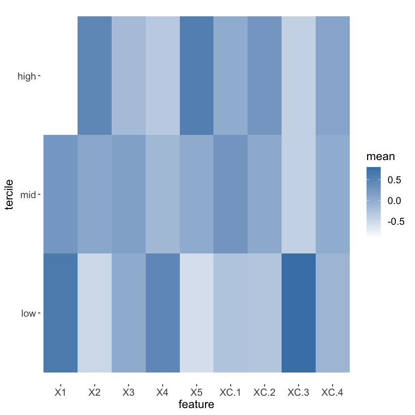
#
# Visualize school-level covariates by treatment heterogeneity
#

school.X.std = scale(school.X)
school.tercile = cut(school.pred,
                     breaks = c(-Inf, quantile(school.pred, c(1/3, 2/3)), Inf))
school.tercile.mat = model.matrix(~ school.tercile + 0)
school.means = diag(1 / colSums(school.tercile.mat)) %*% t(school.tercile.mat) %*% as.matrix(school.X.std)

MM = max(abs(school.means))
HC = heat.colors(21)
school.col = apply(school.means, 1:2, function(aa) HC[1 + round(20 * (0.5 + aa))])

DF.plot = data.frame(tercile=rep(factor(1:3, labels=c("low", "mid", "high")), 9), mean=as.numeric(school.means),
                     feature = factor(rbind(colnames(school.X), colnames(school.X), colnames(school.X))))

ggplot(data = DF.plot, aes(x = feature, y = tercile, fill = mean)) +
    geom_tile() + scale_fill_gradient(low = "white", high = "steelblue") +
    theme(axis.text = element_text(size=12), axis.title = element_text(size=14),
          legend.title = element_text(size=14), legend.text = element_text(size=12)) +
    theme(panel.background = element_blank())
#ggsave("tercile_plot.pdf", width = 8, height = 4.5, dpi = 120)

mean(school.X$XC.3)
mean(school.X$XC.3[as.numeric(school.tercile) == 1])
0.210526315789474
0.538461538461538
#
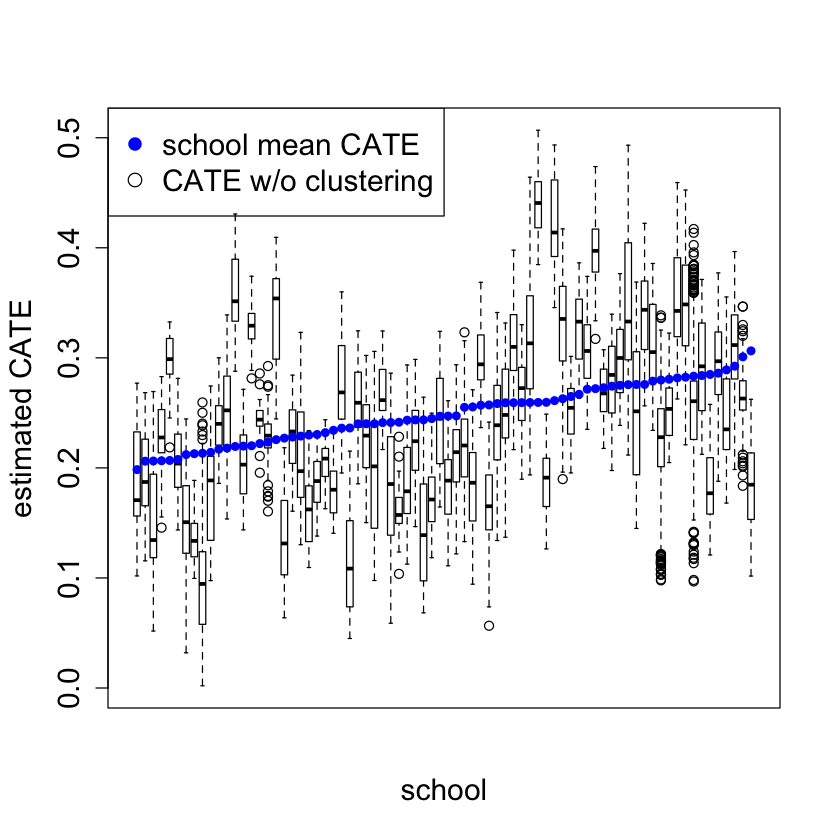
# CATE by school
#
ord = order(order(school.pred))
school.sort = ord[school.id]
#pdf("school_boxplot.pdf")
pardef = par(mar = c(5, 4, 4, 2) + 0.5, cex.lab=1.5, cex.axis=1.5, cex.main=1.5, cex.sub=1.5)
boxplot(tau.hat.noclust ~ school.sort, xaxt = "n",
xlab = "school", ylab = "estimated CATE")
points(1:76, sort(school.pred), col = 4, pch = 16)
legend("topleft", c("school mean CATE", "CATE w/o clustering"), pch = c(16, 1), col = c(4, 1), cex = 1.5)
par = pardef
#dev.off()