词向量模型简介#
Introduction to Word Embeddings: Analyzing Meaning through Word Embeddings
Using vectors to represent things
one of the most fascinating ideas in machine learning.
Word2vec is a method to efficiently create word embeddings.
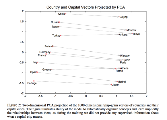
Mikolov et al. (2013). Efficient Estimation of Word Representations in Vector Space
Mikolov et al. (2013). Distributed representations of words and phrases and their compositionality
The Geometry of Culture#
Analyzing Meaning through Word Embeddings
Austin C. Kozlowski; Matt Taddy; James A. Evans
https://arxiv.org/abs/1803.09288
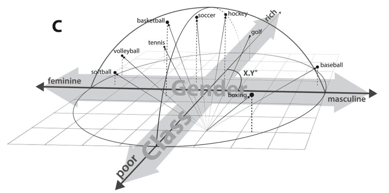
Word embeddings represent semantic relations between words as geometric relationships between vectors in a high-dimensional space, operationalizing a relational model of meaning consistent with contemporary theories of identity and culture.
Dimensions induced by word differences (e.g. man - woman, rich - poor, black - white, liberal - conservative) in these vector spaces closely correspond to dimensions of cultural meaning,
Macro-cultural investigation with a longitudinal analysis of the coevolution of gender and class associations in the United States over the 20th century
The success of these high-dimensional models motivates a move towards “high-dimensional theorizing” of meanings, identities and cultural processes.
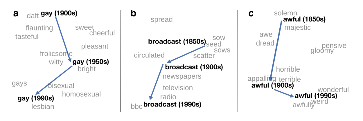
HistWords#
HistWords is a collection of tools and datasets for analyzing language change using word vector embeddings.
The goal of this project is to facilitate quantitative research in diachronic linguistics, history, and the digital humanities.
We used the historical word vectors in HistWords to study the semantic evolution of more than 30,000 words across 4 languages.
This study led us to propose two statistical laws that govern the evolution of word meaning
https://nlp.stanford.edu/projects/histwords/
Diachronic Word Embeddings Reveal Statistical Laws of Semantic Change
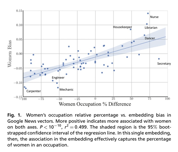
Word embeddings quantify 100 years of gender and ethnic stereotypes#
http://www.pnas.org/content/early/2018/03/30/1720347115
The Illustrated Word2vec#
Jay Alammar. https://jalammar.github.io/illustrated-word2vec/
Personality Embeddings#
What are you like?
Big Five personality traits: openness to experience, conscientiousness, extraversion, agreeableness, and neuroticism
the five-factor model (FFM)
the OCEAN model
开放性(openness):具有想象、审美、情感丰富、求异、创造、智能等特质。
责任心(conscientiousness):显示胜任、公正、条理、尽职、成就、自律、谨慎、克制等特点。
外倾性(extraversion):表现出热情、社交、果断、活跃、冒险、乐观等特质。
宜人性(agreeableness):具有信任、利他、直率、依从、谦虚、移情等特质。
神经质或情绪稳定性(neuroticism):具有平衡焦虑、敌对、压抑、自我意识、冲动、脆弱等情绪的特质,即具有保持情绪稳定的能力。
# Personality Embeddings: What are you like?
jay = [-0.4, 0.8, 0.5, -0.2, 0.3]
john = [-0.3, 0.2, 0.3, -0.4, 0.9]
mike = [-0.5, -0.4, -0.2, 0.7, -0.1]
Cosine Similarity#
The cosine of two non-zero vectors can be derived by using the Euclidean dot product formula:
where \(A_i\) and \(B_i\) are components of vector \(A\) and \(B\) respectively.
from numpy import dot
from numpy.linalg import norm

def cos_sim(a, b):
    return dot(a, b)/(norm(a)*norm(b))

cos_sim([1, 0, -1], [-1,-1, 0])
-0.4999999999999999
from sklearn.metrics.pairwise import cosine_similarity

cosine_similarity([[1, 0, -1]], [[-1,-1, 0]])
array([[-0.5]])
from scipy import spatial
# spatial.distance.cosine computes
# the Cosine distance between 1-D arrays.
1-spatial.distance.cosine([1, 0, -1], [-1,-1, 0])
-0.5
cos_sim(jay, john)
0.6582337075311759
cos_sim(jay, mike)
-0.3683509554826695
Cosine similarity works for any number of dimensions.
We can represent people (and things) as vectors of numbers (which is great for machines!).
We can easily calculate how similar vectors are to each other.
Word Embeddings#
Google News Word2Vec#
You can download Google’s pre-trained model here.
It’s 1.5GB!
It includes word vectors for a vocabulary of 3 million words and phrases
It is trained on roughly 100 billion words from a Google News dataset.
The vector length is 300 features.
http://mccormickml.com/2016/04/12/googles-pretrained-word2vec-model-in-python/
Using the Gensim library in python, we can
find the most similar words to the resulting vector.
add and subtract word vectors,
import gensim
# Load Google's pre-trained Word2Vec model.
filepath = '/Users/datalab/bigdata/GoogleNews-vectors-negative300.bin'
model = gensim.models.KeyedVectors.load_word2vec_format(filepath, binary=True)
model['woman'][:5]
array([ 0.24316406, -0.07714844, -0.10302734, -0.10742188,  0.11816406],
      dtype=float32)
model.most_similar('woman')
[('man', 0.7664012908935547),
 ('girl', 0.7494640946388245),
 ('teenage_girl', 0.7336829900741577),
 ('teenager', 0.631708562374115),
 ('lady', 0.6288785934448242),
 ('teenaged_girl', 0.614178478717804),
 ('mother', 0.6076306104660034),
 ('policewoman', 0.6069462299346924),
 ('boy', 0.5975908637046814),
 ('Woman', 0.5770983099937439)]
model.similarity('woman', 'man')
0.76640123
cos_sim(model['woman'], model['man'])
0.76640123
model.most_similar(positive=['woman', 'king'], negative=['man'], topn=5)
[('queen', 0.7118193507194519),
 ('monarch', 0.6189674735069275),
 ('princess', 0.5902431011199951),
 ('crown_prince', 0.5499460697174072),
 ('prince', 0.5377321243286133)]
model.most_similar(positive=['London', 'China'], negative=['Beijing'], topn=5)
[('UK', 0.6304796934127808),
 ('Britain', 0.6012536287307739),
 ('EURASIAN_NATURAL_RESOURCES_CORP.', 0.5524139404296875),
 ('Europe', 0.5444058775901794),
 ('United_Kingdom', 0.5375455021858215)]
model.most_similar(positive=['big', 'worst'], negative=['bad'], topn=5)
[('biggest', 0.7630176544189453),
 ('greatest', 0.6113720536231995),
 ('major', 0.5540789365768433),
 ('huge', 0.5368192195892334),
 ('Biggest', 0.5305125713348389)]
model.most_similar(positive=['go', 'do'], negative=['did'], topn=5)
[('come', 0.6050394177436829),
 ('get', 0.5739777684211731),
 ('goes', 0.5202917456626892),
 ('happen', 0.5166401267051697),
 ('sit', 0.5145819187164307)]
Now that we’ve looked at trained word embeddings,
let’s learn more about the training process.
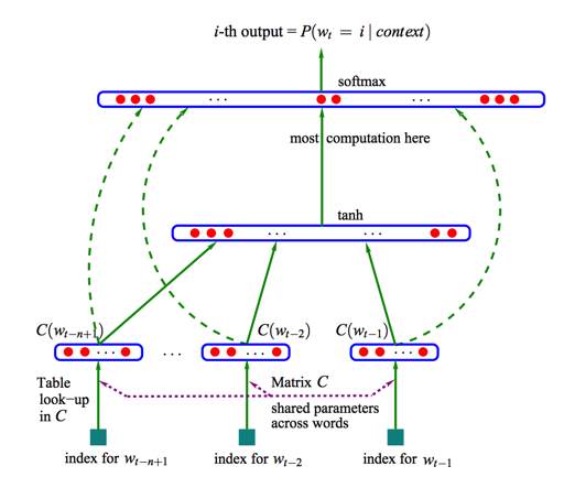
But before we get to word2vec, we need to look at a conceptual parent of word embeddings: the neural language model.
The neural language model#
“You shall know a word by the company it keeps” J.R. Firth
Bengio 2003 A Neural Probabilistic Language Model. Journal of Machine Learning Research. 3:1137–1155
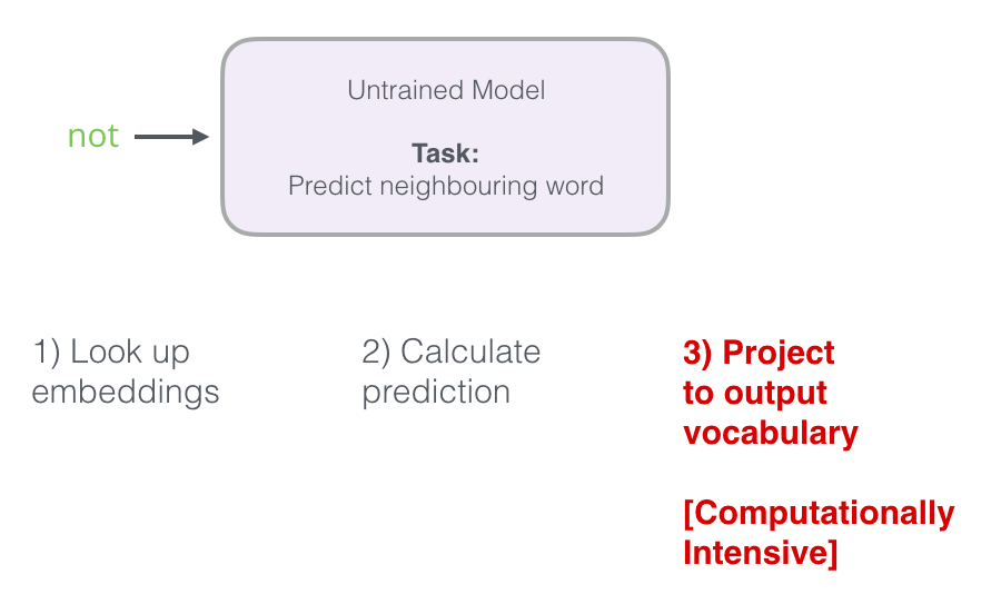
After being trained, early neural language models (Bengio 2003) would calculate a prediction in three steps:
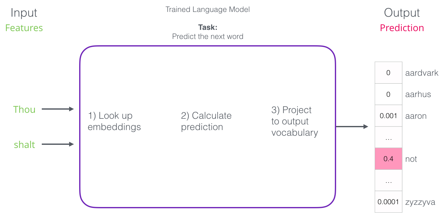
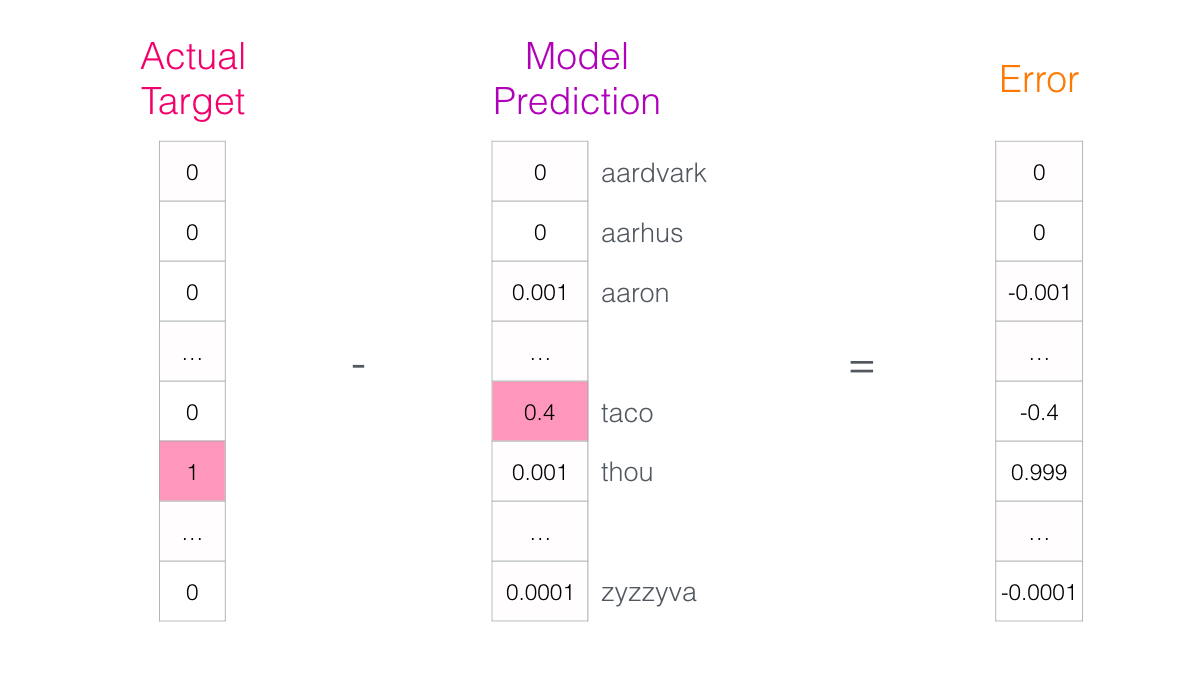
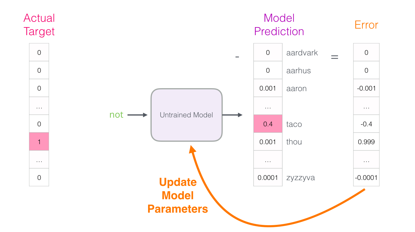
The output of the neural language model is a probability score for all the words the model knows.
We’re referring to the probability as a percentage here,
but 40% would actually be represented as 0.4 in the output vector.
Language Model Training#
We get a lot of text data (say, all Wikipedia articles, for example). then
We have a window (say, of three words) that we slide against all of that text.
The sliding window generates training samples for our model
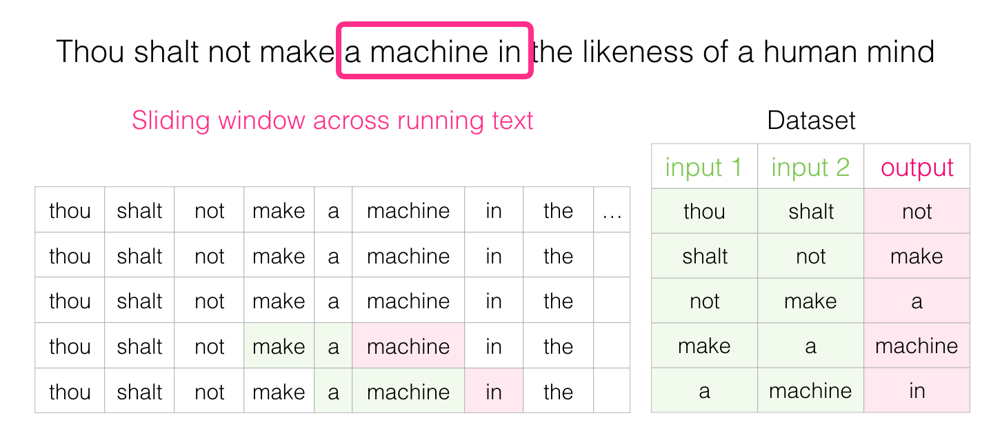
As this window slides against the text, we (virtually) generate a dataset that we use to train a model.
Instead of only looking two words before the target word, we can also look at two words after it.

If we do this, the dataset we’re virtually building and training the model against would look like this:
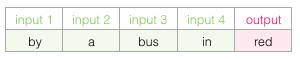
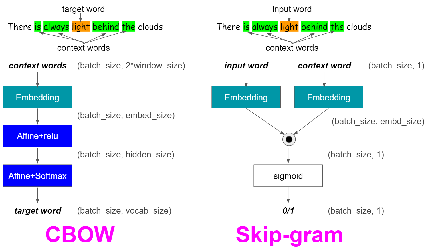
This is called a Continuous Bag of Words (CBOW) https://arxiv.org/pdf/1301.3781.pdf
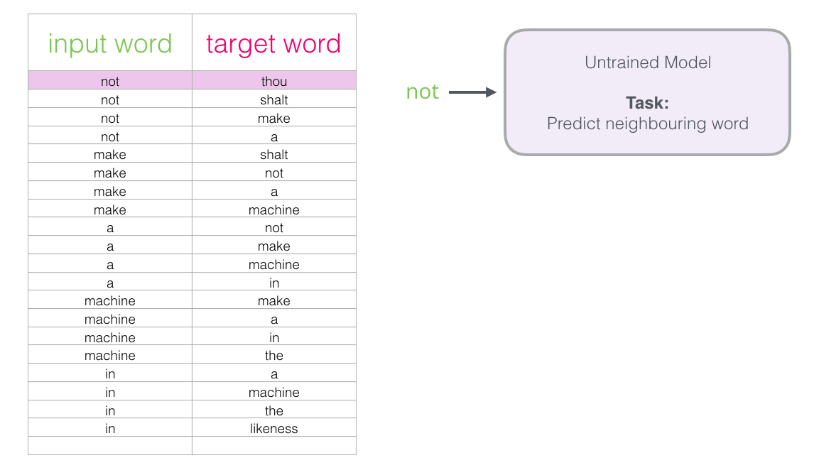
Skip-gram#
Instead of guessing a word based on its context (the words before and after it), this other architecture tries to guess neighboring words using the current word.
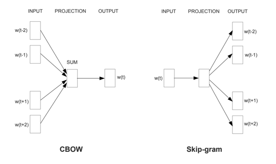
https://arxiv.org/pdf/1301.3781.pdf
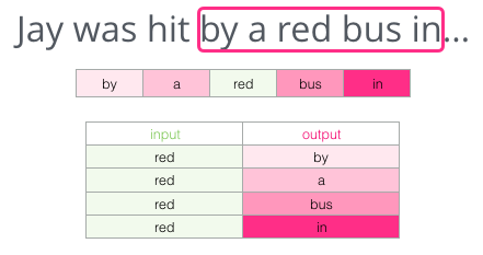
The pink boxes are in different shades because this sliding window actually creates four separate samples in our training dataset.
We then slide our window to the next position:
Which generates our next four examples:
Negative Sampling#
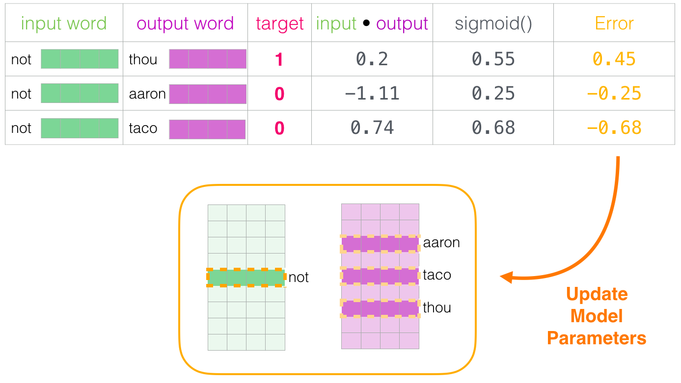
And switch it to a model that takes the input and output word, and outputs a score indicating if they’re neighbors or not
0 for “not neighbors”, 1 for “neighbors”.
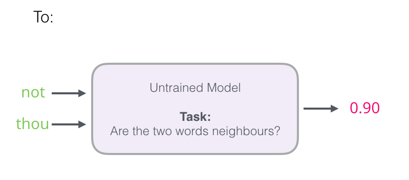
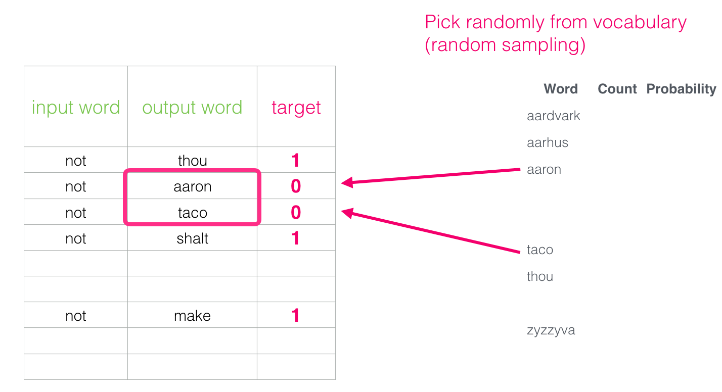
we need to introduce negative samples to our dataset
samples of words that are not neighbors.
Our model needs to return 0 for those samples.
This leads to a great tradeoff of computational and statistical efficiency.
Skipgram with Negative Sampling (SGNS)
Word2vec Training Process#
Pytorch word2vec#
# see http://pytorch.org/tutorials/beginner/nlp/word_embeddings_tutorial.html
import torch
from torch.autograd import Variable
import torch.nn as nn
import torch.nn.functional as F
import torch.optim as optim

torch.manual_seed(1)
<torch._C.Generator at 0x116c571d0>
text = """We are about to study the idea of a computational process.
Computational processes are abstract beings that inhabit computers.
As they evolve, processes manipulate other abstract things called data.
The evolution of a process is directed by a pattern of rules
called a program. People create programs to direct processes. In effect,
we conjure the spirits of the computer with our spells."""

text = text.replace(',', '').replace('.', '').lower().split()
# By deriving a set from `raw_text`, we deduplicate the array
vocab = set(text)
vocab_size = len(vocab)
print('vocab_size:', vocab_size)

w2i = {w: i for i, w in enumerate(vocab)}
i2w = {i: w for i, w in enumerate(vocab)}
vocab_size: 44
# context window size is two
def create_cbow_dataset(text):
    data = []
    for i in range(2, len(text) - 2):
        context = [text[i - 2], text[i - 1],
                   text[i + 1], text[i + 2]]
        target = text[i]
        data.append((context, target))
    return data

cbow_train = create_cbow_dataset(text)
print('cbow sample', cbow_train[0])
cbow sample (['we', 'are', 'to', 'study'], 'about')
def create_skipgram_dataset(text):
    import random
    data = []
    for i in range(2, len(text) - 2):
        data.append((text[i], text[i-2], 1))
        data.append((text[i], text[i-1], 1))
        data.append((text[i], text[i+1], 1))
        data.append((text[i], text[i+2], 1))
        # negative sampling
        for _ in range(4):
            if random.random() < 0.5 or i >= len(text) - 3:
                rand_id = random.randint(0, i-1)
            else:
                rand_id = random.randint(i+3, len(text)-1)
            data.append((text[i], text[rand_id], 0))
    return data


skipgram_train = create_skipgram_dataset(text)
print('skipgram sample', skipgram_train[0])
skipgram sample ('about', 'we', 1)
class CBOW(nn.Module):
    def __init__(self, vocab_size, embd_size, context_size, hidden_size):
        super(CBOW, self).__init__()
        self.embeddings = nn.Embedding(vocab_size, embd_size)
        self.linear1 = nn.Linear(2*context_size*embd_size, hidden_size)
        self.linear2 = nn.Linear(hidden_size, vocab_size)

    def forward(self, inputs):
        embedded = self.embeddings(inputs).view((1, -1))
        hid = F.relu(self.linear1(embedded))
        out = self.linear2(hid)
        log_probs = F.log_softmax(out, dim = 1)
        return log_probs

    def extract(self, inputs):
        embeds = self.embeddings(inputs)
        return embeds
class SkipGram(nn.Module):
    def __init__(self, vocab_size, embd_size):
        super(SkipGram, self).__init__()
        self.embeddings = nn.Embedding(vocab_size, embd_size)

    def forward(self, focus, context):
        embed_focus = self.embeddings(focus).view((1, -1)) # input
        embed_ctx = self.embeddings(context).view((1, -1)) # output
        score = torch.mm(embed_focus, torch.t(embed_ctx)) # input*output
        log_probs = F.logsigmoid(score) # sigmoid
        return log_probs

    def extract(self, focus):
        embed_focus = self.embeddings(focus)
        return embed_focus
torch.mm Performs a matrix multiplication of the matrices
torch.t Expects :attr:input to be a matrix (2-D tensor) and transposes dimensions 0
and 1. Can be seen as a short-hand function for transpose(input, 0, 1).
embd_size = 100
learning_rate = 0.001
n_epoch = 30
CONTEXT_SIZE = 2  # 2 words to the left, 2 to the right
def train_cbow():
    hidden_size = 64
    losses = []
    loss_fn = nn.NLLLoss()
    model = CBOW(vocab_size, embd_size, CONTEXT_SIZE, hidden_size)
    print(model)
    optimizer = optim.SGD(model.parameters(), lr=learning_rate)
    for epoch in range(n_epoch):
        total_loss = .0
        for context, target in cbow_train:
            ctx_idxs = [w2i[w] for w in context]
            ctx_var = Variable(torch.LongTensor(ctx_idxs))

            model.zero_grad()
            log_probs = model(ctx_var)

            loss = loss_fn(log_probs, Variable(torch.LongTensor([w2i[target]])))

            loss.backward()
            optimizer.step()

            total_loss += loss.data.item()
        losses.append(total_loss)
    return model, losses
def train_skipgram():
    losses = []
    loss_fn = nn.MSELoss()
    model = SkipGram(vocab_size, embd_size)
    print(model)
    optimizer = optim.SGD(model.parameters(), lr=learning_rate)

    for epoch in range(n_epoch):
        total_loss = .0
        for in_w, out_w, target in skipgram_train:
            in_w_var = Variable(torch.LongTensor([w2i[in_w]]))
            out_w_var = Variable(torch.LongTensor([w2i[out_w]]))

            model.zero_grad()
            log_probs = model(in_w_var, out_w_var)
            loss = loss_fn(log_probs[0], Variable(torch.Tensor([target])))

            loss.backward()
            optimizer.step()

            total_loss += loss.data.item()
        losses.append(total_loss)
    return model, losses
cbow_model, cbow_losses = train_cbow()
sg_model, sg_losses = train_skipgram()
CBOW(
  (embeddings): Embedding(44, 100)
  (linear1): Linear(in_features=400, out_features=64, bias=True)
  (linear2): Linear(in_features=64, out_features=44, bias=True)
)
SkipGram(
  (embeddings): Embedding(44, 100)
)
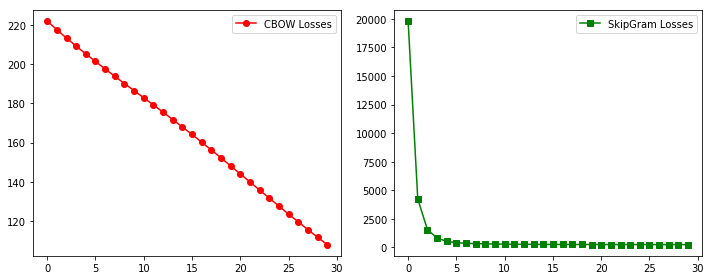
plt.figure(figsize= (10, 4))
plt.subplot(121)
plt.plot(range(n_epoch), cbow_losses, 'r-o', label = 'CBOW Losses')
plt.legend()
plt.subplot(122)
plt.plot(range(n_epoch), sg_losses, 'g-s', label = 'SkipGram Losses')
plt.legend()
plt.tight_layout()
cbow_vec = cbow_model.extract(Variable(torch.LongTensor([v for v in w2i.values()])))
cbow_vec = cbow_vec.data.numpy()
len(cbow_vec[0])
100
sg_vec = sg_model.extract(Variable(torch.LongTensor([v for v in w2i.values()])))
sg_vec = sg_vec.data.numpy()
len(sg_vec[0])
100
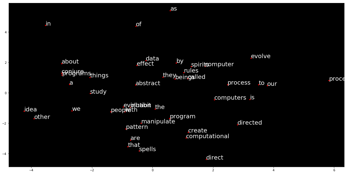
# 利用PCA算法进行降维
from sklearn.decomposition import PCA
X_reduced = PCA(n_components=2).fit_transform(sg_vec)

# 绘制所有单词向量的二维空间投影
import matplotlib.pyplot as plt
import matplotlib

fig = plt.figure(figsize = (20, 10))
ax = fig.gca()
ax.set_facecolor('black')
ax.plot(X_reduced[:, 0], X_reduced[:, 1], '.', markersize = 1, alpha = 0.4, color = 'white')
# 绘制几个特殊单词的向量
words = list(w2i.keys())
# 设置中文字体,否则无法在图形上显示中文
for w in words:
    if w in w2i:
        ind = w2i[w]
        xy = X_reduced[ind]
        plt.plot(xy[0], xy[1], '.', alpha =1, color = 'red')
        plt.text(xy[0], xy[1], w, alpha = 1, color = 'white', fontsize = 20)
NGram词向量模型#
本文件是集智AI学园http://campus.swarma.org 出品的“火炬上的深度学习”第VI课的配套源代码
原理:利用一个人工神经网络来根据前N个单词来预测下一个单词,从而得到每个单词的词向量
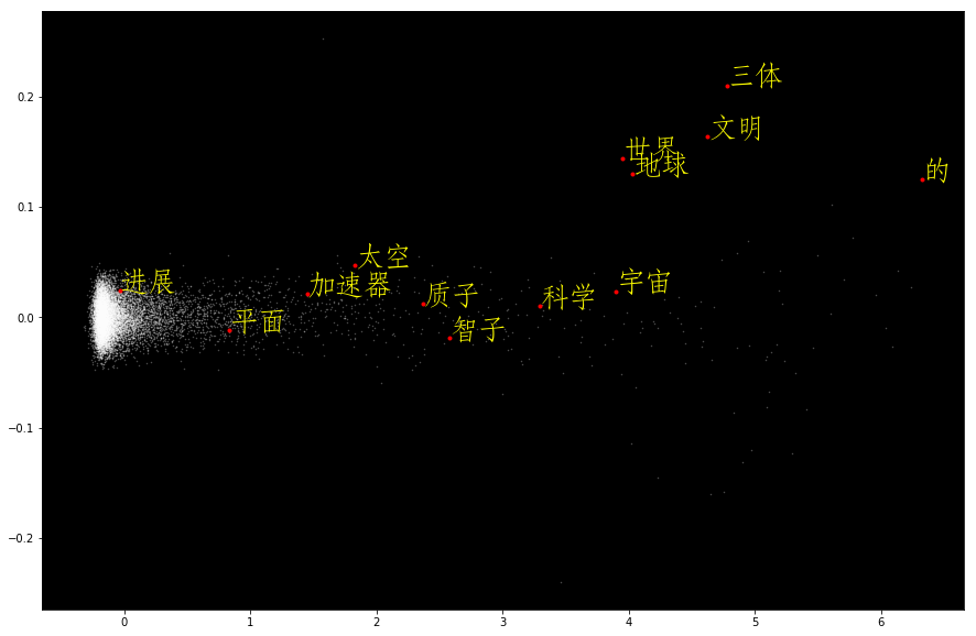
以刘慈欣著名的科幻小说《三体》为例,来展示利用NGram模型训练词向量的方法
预处理分为两个步骤:1、读取文件、2、分词、3、将语料划分为N+1元组,准备好训练用数据
在这里,我们并没有去除标点符号,一是为了编程简洁,而是考虑到分词会自动将标点符号当作一个单词处理,因此不需要额外考虑。
with open("../data/3body.txt", 'r') as f:
    text = str(f.read())
import jieba, re
temp = jieba.lcut(text)
words = []
for i in temp:
    #过滤掉所有的标点符号
    i = re.sub("[\s+\.\!\/_,$%^*(+\"\'””《》]+|[+——!,。?、~@#¥%……&*():]+", "", i)
    if len(i) > 0:
        words.append(i)
print(len(words))
7754
text[:100]
'八万五千三体时(约8.6个地球年)后。\n\n元首下令召开三体世界全体执政官紧急会议,这很不寻常,一定有什么重大的事件发生。\n\n两万三体时前,三体舰队启航了,它们只知道目标的大致方向,却不知道它的距离。也'
print(*words[:50])
八万五千 三体 时 约 86 个 地球 年 后 元首 下令 召开 三体 世界 全体 执政官 紧急会议 这 很 不 寻常 一定 有 什么 重大 的 事件 发生 两万 三体 时前 三体 舰队 启航 了 它们 只 知道 目标 的 大致 方向 却 不 知道 它 的 距离 也许 目标
trigrams = [([words[i], words[i + 1]], words[i + 2]) for i in range(len(words) - 2)]
# 打印出前三个元素看看
print(trigrams[:3])
[(['八万五千', '三体'], '时'), (['三体', '时'], '约'), (['时', '约'], '86')]
# 得到词汇表
vocab = set(words)
print(len(vocab))
word_to_idx = {i:[k, 0] for k, i in enumerate(vocab)}
idx_to_word = {k:i for k, i in enumerate(vocab)}
for w in words:
     word_to_idx[w][1] +=1
2000
构造NGram神经网络模型 (三层的网络)
输入层:embedding层,这一层的作用是:先将输入单词的编号映射为一个one hot编码的向量,形如:001000,维度为单词表大小。 然后,embedding会通过一个线性的神经网络层映射到这个词的向量表示,输出为embedding_dim
线性层,从embedding_dim维度到128维度,然后经过非线性ReLU函数
线性层:从128维度到单词表大小维度,然后log softmax函数,给出预测每个单词的概率
import torch.nn as nn
import torch.nn.functional as F
import torch.optim as optim
from torch.autograd import Variable

import torch

class NGram(nn.Module):
    def __init__(self, vocab_size, embedding_dim, context_size):
        super(NGram, self).__init__()
        self.embeddings = nn.Embedding(vocab_size, embedding_dim)  #嵌入层
        self.linear1 = nn.Linear(context_size * embedding_dim, 128) #线性层
        self.linear2 = nn.Linear(128, vocab_size) #线性层

    def forward(self, inputs):
        #嵌入运算,嵌入运算在内部分为两步:将输入的单词编码映射为one hot向量表示,然后经过一个线性层得到单词的词向量
        embeds = self.embeddings(inputs).view(1, -1)
        # 线性层加ReLU
        out = F.relu(self.linear1(embeds))

        # 线性层加Softmax
        out = self.linear2(out)
        log_probs = F.log_softmax(out, dim = 1)
        return log_probs
    def extract(self, inputs):
        embeds = self.embeddings(inputs)
        return embeds
losses = [] #纪录每一步的损失函数
criterion = nn.NLLLoss() #运用负对数似然函数作为目标函数(常用于多分类问题的目标函数)
model = NGram(len(vocab), 10, 2) #定义NGram模型,向量嵌入维数为10维,N(窗口大小)为2
optimizer = optim.SGD(model.parameters(), lr=0.001) #使用随机梯度下降算法作为优化器
#循环100个周期
for epoch in range(100):
    total_loss = torch.Tensor([0])
    for context, target in trigrams:
        # 准备好输入模型的数据,将词汇映射为编码
        context_idxs = [word_to_idx[w][0] for w in context]
        # 包装成PyTorch的Variable
        context_var = Variable(torch.LongTensor(context_idxs))
        # 清空梯度:注意PyTorch会在调用backward的时候自动积累梯度信息,故而每隔周期要清空梯度信息一次。
        optimizer.zero_grad()
        # 用神经网络做计算,计算得到输出的每个单词的可能概率对数值
        log_probs = model(context_var)
        # 计算损失函数,同样需要把目标数据转化为编码,并包装为Variable
        loss = criterion(log_probs, Variable(torch.LongTensor([word_to_idx[target][0]])))
        # 梯度反传
        loss.backward()
        # 对网络进行优化
        optimizer.step()
        # 累加损失函数值
        total_loss += loss.data
    losses.append(total_loss)
    print('第{}轮,损失函数为:{:.2f}'.format(epoch, total_loss.numpy()[0]))
第0轮,损失函数为:56704.61
第1轮,损失函数为:53935.28
第2轮,损失函数为:52241.16
第3轮,损失函数为:51008.51
第4轮,损失函数为:50113.76
第5轮,损失函数为:49434.07
第6轮,损失函数为:48879.33
第7轮,损失函数为:48404.71
第8轮,损失函数为:47983.95
第9轮,损失函数为:47600.01
第10轮,损失函数为:47240.32
第11轮,损失函数为:46897.53
第12轮,损失函数为:46566.24
第13轮,损失函数为:46241.59
第14轮,损失函数为:45920.18
第15轮,损失函数为:45599.50
第16轮,损失函数为:45277.74
第17轮,损失函数为:44953.10
第18轮,损失函数为:44624.41
第19轮,损失函数为:44290.34
第20轮,损失函数为:43950.63
第21轮,损失函数为:43604.48
第22轮,损失函数为:43251.90
第23轮,损失函数为:42891.99
第24轮,损失函数为:42524.64
第25轮,损失函数为:42149.46
第26轮,损失函数为:41766.14
第27轮,损失函数为:41374.89
第28轮,损失函数为:40975.62
第29轮,损失函数为:40568.36
第30轮,损失函数为:40153.31
第31轮,损失函数为:39730.61
第32轮,损失函数为:39300.70
第33轮,损失函数为:38863.39
第34轮,损失函数为:38419.11
第35轮,损失函数为:37968.16
第36轮,损失函数为:37510.99
第37轮,损失函数为:37048.06
第38轮,损失函数为:36579.82
第39轮,损失函数为:36106.78
第40轮,损失函数为:35629.46
第41轮,损失函数为:35148.57
第42轮,损失函数为:34665.39
第43轮,损失函数为:34180.25
第44轮,损失函数为:33693.93
第45轮,损失函数为:33207.48
第46轮,损失函数为:32721.72
第47轮,损失函数为:32237.36
第48轮,损失函数为:31755.00
第49轮,损失函数为:31275.05
第50轮,损失函数为:30798.38
第51轮,损失函数为:30325.62
第52轮,损失函数为:29857.59
第53轮,损失函数为:29394.65
第54轮,损失函数为:28937.08
第55轮,损失函数为:28485.72
第56轮,损失函数为:28041.07
第57轮,损失函数为:27603.33
第58轮,损失函数为:27173.14
第59轮,损失函数为:26750.82
第60轮,损失函数为:26336.92
第61轮,损失函数为:25931.60
第62轮,损失函数为:25534.87
第63轮,损失函数为:25147.07
第64轮,损失函数为:24768.02
第65轮,损失函数为:24397.92
第66轮,损失函数为:24036.68
第67轮,损失函数为:23684.69
第68轮,损失函数为:23341.30
第69轮,损失函数为:23006.46
第70轮,损失函数为:22680.18
第71轮,损失函数为:22361.95
第72轮,损失函数为:22051.86
第73轮,损失函数为:21749.46
第74轮,损失函数为:21454.48
第75轮,损失函数为:21167.06
第76轮,损失函数为:20886.72
第77轮,损失函数为:20613.04
第78轮,损失函数为:20346.13
第79轮,损失函数为:20085.52
第80轮,损失函数为:19831.27
第81轮,损失函数为:19583.16
第82轮,损失函数为:19341.03
第83轮,损失函数为:19104.43
第84轮,损失函数为:18873.11
第85轮,损失函数为:18646.91
第86轮,损失函数为:18425.87
第87轮,损失函数为:18209.80
第88轮,损失函数为:17998.34
第89轮,损失函数为:17791.97
第90轮,损失函数为:17589.94
第91轮,损失函数为:17392.24
第92轮,损失函数为:17199.04
第93轮,损失函数为:17009.97
第94轮,损失函数为:16824.82
第95轮,损失函数为:16643.87
第96轮,损失函数为:16466.76
第97轮,损失函数为:16293.54
第98轮,损失函数为:16123.99
第99轮,损失函数为:15957.75
12m 24s!!!
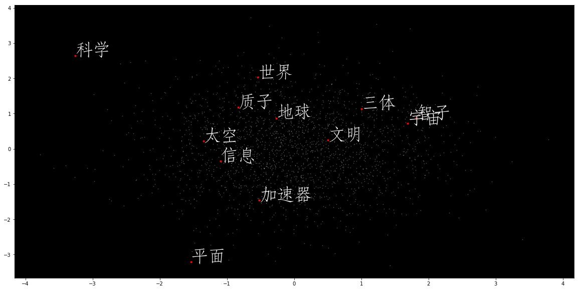
# 从训练好的模型中提取每个单词的向量
vec = model.extract(Variable(torch.LongTensor([v[0] for v in word_to_idx.values()])))
vec = vec.data.numpy()

# 利用PCA算法进行降维
from sklearn.decomposition import PCA
X_reduced = PCA(n_components=2).fit_transform(vec)
# 绘制所有单词向量的二维空间投影
import matplotlib.pyplot as plt
import matplotlib

fig = plt.figure(figsize = (20, 10))
ax = fig.gca()
ax.set_facecolor('black')
ax.plot(X_reduced[:, 0], X_reduced[:, 1], '.', markersize = 1, alpha = 0.4, color = 'white')
# 绘制几个特殊单词的向量
words = ['智子', '地球', '三体', '质子', '科学', '世界', '文明', '太空', '加速器', '平面', '宇宙', '信息']
# 设置中文字体,否则无法在图形上显示中文
zhfont1 = matplotlib.font_manager.FontProperties(fname='/Library/Fonts/华文仿宋.ttf', size = 35)
for w in words:
    if w in word_to_idx:
        ind = word_to_idx[w][0]
        xy = X_reduced[ind]
        plt.plot(xy[0], xy[1], '.', alpha =1, color = 'red')
        plt.text(xy[0], xy[1], w, fontproperties = zhfont1, alpha = 1, color = 'white')
# 定义计算cosine相似度的函数
import numpy as np
def cos_similarity(vec1, vec2):
    norm1 = np.linalg.norm(vec1)
    norm2 = np.linalg.norm(vec2)
    norm = norm1 * norm2
    dot = np.dot(vec1, vec2)
    result = dot / norm if norm > 0 else 0
    return result

# 在所有的词向量中寻找到与目标词(word)相近的向量,并按相似度进行排列
def find_most_similar(word, vectors, word_idx):
    vector = vectors[word_to_idx[word][0]]
    simi = [[cos_similarity(vector, vectors[num]), key] for num, key in enumerate(word_idx.keys())]
    sort = sorted(simi)[::-1]
    words = [i[1] for i in sort]
    return words

# 与智子靠近的词汇
find_most_similar('智子', vec, word_to_idx)[:10]
['局部', '一场', '来', '错误', '一生', '正中', '航行', '地面', '只是', '政府']
Gensim Word2vec#
import gensim as gensim
from gensim.models import Word2Vec
from gensim.models.keyedvectors import KeyedVectors
from gensim.models.word2vec import LineSentence
f = open("./data/三体.txt", 'r')
lines = []

import jieba
import re

for line in f:
    temp = jieba.lcut(line)
    words = []
    for i in temp:
        #过滤掉所有的标点符号
        i = re.sub("[\s+\.\!\/_,$%^*(+\"\'””《》]+|[+——!,。?、~@#¥%……&*():;‘]+", "", i)
        if len(i) > 0:
            words.append(i)
    if len(words) > 0:
        lines.append(words)
Building prefix dict from the default dictionary ...
Loading model from cache /var/folders/8b/hhnbt0nd4zsg2qhxc28q23w80000gn/T/jieba.cache
Loading model cost 0.685 seconds.
Prefix dict has been built successfully.
# 调用gensim Word2Vec的算法进行训练。
# 参数分别为:size: 嵌入后的词向量维度;window: 上下文的宽度,min_count为考虑计算的单词的最低词频阈值
model = Word2Vec(lines, vector_size = 20, window = 2 , min_count = 0)
model.wv.most_similar('三体', topn = 100)
[('地球', 0.9974961876869202),
 ('外星', 0.9959420561790466),
 ('中', 0.9958519339561462),
 ('的', 0.9958161115646362),
 ('信息', 0.9955942034721375),
 ('文明', 0.9955913424491882),
 ('时间', 0.9953882694244385),
 ('宇宙', 0.9951216578483582),
 ('发展', 0.9950591325759888),
 ('与', 0.9950133562088013),
 ('一个', 0.9949650764465332),
 ('它', 0.9945959448814392),
 ('四个', 0.9944809079170227),
 ('世界', 0.9944674968719482),
 ('加速器', 0.9942856431007385),
 ('太阳', 0.9941897988319397),
 ('通过', 0.9940699934959412),
 ('放到', 0.9940448999404907),
 ('将', 0.9940245151519775),
 ('社会', 0.9938994646072388),
 ('实验', 0.9938514232635498),
 ('目前', 0.993848979473114),
 ('其他', 0.9938352704048157),
 ('结构', 0.9938239455223083),
 ('存在', 0.9937348961830139),
 ('舰队', 0.9936554431915283),
 ('这个', 0.9936324954032898),
 ('历史', 0.993557333946228),
 ('内', 0.9935263991355896),
 ('使', 0.9934986233711243),
 ('巨大', 0.9934812188148499),
 ('出现', 0.9934180974960327),
 ('最近', 0.9934037327766418),
 ('大殿', 0.9933778047561646),
 ('毁灭', 0.993355929851532),
 ('等', 0.9933347105979919),
 ('在', 0.9933309555053711),
 ('这样', 0.9933069944381714),
 ('而', 0.9932495355606079),
 ('杨冬', 0.9932450652122498),
 ('周围', 0.9932316541671753),
 ('那个', 0.9932215213775635),
 ('产生', 0.9931648373603821),
 ('为', 0.9931637644767761),
 ('所有', 0.9931597113609314),
 ('沙瑞山', 0.9931430220603943),
 ('不同', 0.9931164383888245),
 ('你们', 0.9930866360664368),
 ('人们', 0.993083119392395),
 ('上', 0.993078351020813),
 ('人类', 0.9930549263954163),
 ('人', 0.9930544495582581),
 ('时', 0.9930477142333984),
 ('那些', 0.9930435419082642),
 ('一些', 0.9930272698402405),
 ('该', 0.9929757714271545),
 ('频率', 0.9928855895996094),
 ('技术', 0.9928467273712158),
 ('美好', 0.9928457736968994),
 ('主要', 0.9928236603736877),
 ('疯狂', 0.9928078055381775),
 ('努力', 0.9927535653114319),
 ('进行', 0.9927522540092468),
 ('需要', 0.992743730545044),
 ('被', 0.9927397966384888),
 ('发生', 0.992729127407074),
 ('接触', 0.9927168488502502),
 ('复杂', 0.99271559715271),
 ('研究', 0.9927100539207458),
 ('和', 0.9926401376724243),
 ('于', 0.992630660533905),
 ('发出', 0.9926106333732605),
 ('三', 0.9926024675369263),
 ('运动', 0.9925642013549805),
 ('只能', 0.9925564527511597),
 ('一片', 0.9925556182861328),
 ('已经', 0.9925482273101807),
 ('自己', 0.992435872554779),
 ('计算', 0.9924312829971313),
 ('那样', 0.9924249649047852),
 ('这些', 0.9924024343490601),
 ('第一次', 0.9923712611198425),
 ('一张', 0.9923089742660522),
 ('基地', 0.9922966361045837),
 ('辐射', 0.9922692775726318),
 ('混乱', 0.9922570586204529),
 ('一名', 0.9922410249710083),
 ('其', 0.9922134280204773),
 ('比', 0.9921837449073792),
 ('为了', 0.992165744304657),
 ('计算机', 0.9921648502349854),
 ('个', 0.99213045835495),
 ('天线', 0.9921154975891113),
 ('之间', 0.9921114444732666),
 ('两次', 0.9920859336853027),
 ('建造', 0.9920815825462341),
 ('杨母', 0.9920707941055298),
 ('后面', 0.9920520186424255),
 ('接收', 0.9920087456703186),
 ('如何', 0.9919811487197876)]
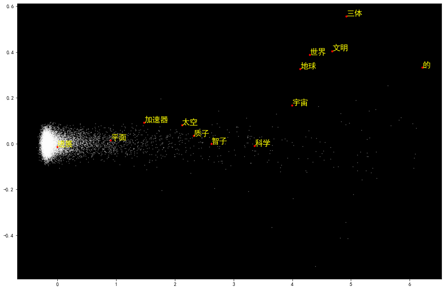
# 将词向量投影到二维空间
import numpy as np
from sklearn.decomposition import PCA

rawWordVec = []
word2ind = {}
for i, w in enumerate(model.wv.key_to_index):
    rawWordVec.append(model.wv[w])
    word2ind[w] = i
rawWordVec = np.array(rawWordVec)
X_reduced = PCA(n_components=2).fit_transform(rawWordVec)
# 绘制星空图
# 绘制所有单词向量的二维空间投影
import matplotlib.pyplot as plt
import matplotlib
plt.rcParams['font.sans-serif'] = ['SimHei']  # 用来正常显示中文标签
plt.rcParams['axes.unicode_minus'] = False  # 用来正常显示负号

fig = plt.figure(figsize = (15, 10))
ax = fig.gca()
ax.set_facecolor('black')
ax.plot(X_reduced[:, 0], X_reduced[:, 1], '.', markersize = 1, alpha = 0.5, color = 'white')
# 绘制几个特殊单词的向量
words = ['智子', '地球', '三体', '质子', '科学', '世界', '文明', '太空', '加速器', '平面', '宇宙', '进展','的']
# 设置中文字体,否则无法在图形上显示中文
#zhfont1 = matplotlib.font_manager.FontProperties(fname='/Library/Fonts/华文仿宋.ttf', size=26)
for w in words:
    if w in word2ind:
        ind = word2ind[w]
        xy = X_reduced[ind]
        plt.plot(xy[0], xy[1], '.', alpha =1, color = 'red')
        #plt.text(xy[0], xy[1], w, fontproperties = zhfont1, alpha = 1, color = 'yellow')
        plt.text(xy[0], xy[1], w, alpha = 1, color = 'yellow', fontsize = 16)
# 绘制星空图
# 绘制所有单词向量的二维空间投影
fig = plt.figure(figsize = (15, 10))
ax = fig.gca()
ax.set_facecolor('black')
ax.plot(X_reduced[:, 0], X_reduced[:, 1], '.', markersize = 1, alpha = 0.3, color = 'white')
# 绘制几个特殊单词的向量
words = ['智子', '地球', '三体', '质子', '科学', '世界', '文明', '太空', '加速器', '平面', '宇宙', '进展','的']
# 设置中文字体,否则无法在图形上显示中文
zhfont1 = matplotlib.font_manager.FontProperties(fname='/Library/Fonts/华文仿宋.ttf', size=26)
for w in words:
    if w in word2ind:
        ind = word2ind[w]
        xy = X_reduced[ind]
        plt.plot(xy[0], xy[1], '.', alpha =1, color = 'red')
        plt.text(xy[0], xy[1], w, fontproperties = zhfont1, alpha = 1, color = 'yellow')