Simulating Network Diffusion With NDlib#

NDlib is a Python language software package for the describing, simulate, and study diffusion processes on complex networks.
NDlib is built upon the NetworkX python library and is intended to provide:
tools for the study diffusion dynamics on social, biological, and infrastructure networks,
a standard programming interface and diffusion models
implementation that is suitable for many applications, a rapid development environment for collaborative, multidisciplinary, projects.
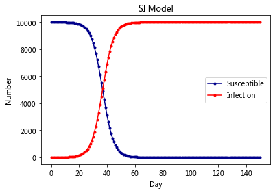
The SI Model#

Given every individual in the system must be either susceptible or infected, \(I + S = 1\). Thus, the equations above can be transformed to:
To solve this differential equation, we can get the cumulative growth curve as a function of time:
Interestingly, this is a logistic growth featured by its S-shaped curve. The curve grows exponentially shortly after the system is infected, and then saturates as the number of susceptible shrinks which makes it harder to find the next victims.
from sympy import dsolve, Eq, symbols, Function

t = symbols('t')
b = symbols('b')
I = symbols('I', cls=Function)
deqn1 = Eq(I(t).diff(t), b*I(t)*(1 - I(t)))
dsolve(deqn1, I(t))
import scipy.integrate as spi
import numpy as np
import matplotlib.pyplot as plt
# Integrate a system of ordinary differential equations.
# Solves the initial value problem for stiff or non-stiff systems
# of first order ode-s::
# dy/dt = func(y, t, ...)  [or func(t, y, ...)]
spi.odeint?
# N为人群总数
N = 10000
# β为传染率系数
beta = 0.25
# I_0为感染者的初始人数
I_0 = 1
# S_0为易感者的初始人数
S_0 = N - I_0
# T为传播时间
T = 150
def funcSI(inivalue,_):
    # inivalue = (S_0,I_0)
    Y = np.zeros(2)
    X = inivalue
    # 易感个体变化
    Y[0] = - (beta * X[0] * X[1]) / N
    # 感染个体变化
    Y[1] = (beta * X[0] * X[1]) / N
    return Y

# INI为初始状态下的数组
INI = (S_0,I_0)
T_range = np.arange(0,T + 1)
RES = spi.odeint(funcSI,INI,T_range)
help(spi.odeint)
Help on function odeint in module scipy.integrate.odepack:

odeint(func, y0, t, args=(), Dfun=None, col_deriv=0, full_output=0, ml=None, mu=None, rtol=None, atol=None, tcrit=None, h0=0.0, hmax=0.0, hmin=0.0, ixpr=0, mxstep=0, mxhnil=0, mxordn=12, mxords=5, printmessg=0, tfirst=False)
    Integrate a system of ordinary differential equations.

    .. note:: For new code, use `scipy.integrate.solve_ivp` to solve a
              differential equation.

    Solve a system of ordinary differential equations using lsoda from the
    FORTRAN library odepack.

    Solves the initial value problem for stiff or non-stiff systems
    of first order ode-s::

        dy/dt = func(y, t, ...)  [or func(t, y, ...)]

    where y can be a vector.

    .. note:: By default, the required order of the first two arguments of
              `func` are in the opposite order of the arguments in the system
              definition function used by the `scipy.integrate.ode` class and
              the function `scipy.integrate.solve_ivp`.  To use a function with
              the signature ``func(t, y, ...)``, the argument `tfirst` must be
              set to ``True``.

    Parameters
    ----------
    func : callable(y, t, ...) or callable(t, y, ...)
        Computes the derivative of y at t.
        If the signature is ``callable(t, y, ...)``, then the argument
        `tfirst` must be set ``True``.
    y0 : array
        Initial condition on y (can be a vector).
    t : array
        A sequence of time points for which to solve for y.  The initial
        value point should be the first element of this sequence.
        This sequence must be monotonically increasing or monotonically
        decreasing; repeated values are allowed.
    args : tuple, optional
        Extra arguments to pass to function.
    Dfun : callable(y, t, ...) or callable(t, y, ...)
        Gradient (Jacobian) of `func`.
        If the signature is ``callable(t, y, ...)``, then the argument
        `tfirst` must be set ``True``.
    col_deriv : bool, optional
        True if `Dfun` defines derivatives down columns (faster),
        otherwise `Dfun` should define derivatives across rows.
    full_output : bool, optional
        True if to return a dictionary of optional outputs as the second output
    printmessg : bool, optional
        Whether to print the convergence message
    tfirst: bool, optional
        If True, the first two arguments of `func` (and `Dfun`, if given)
        must ``t, y`` instead of the default ``y, t``.

        .. versionadded:: 1.1.0

    Returns
    -------
    y : array, shape (len(t), len(y0))
        Array containing the value of y for each desired time in t,
        with the initial value `y0` in the first row.
    infodict : dict, only returned if full_output == True
        Dictionary containing additional output information

        =======  ============================================================
        key      meaning
        =======  ============================================================
        'hu'     vector of step sizes successfully used for each time step.
        'tcur'   vector with the value of t reached for each time step.
                 (will always be at least as large as the input times).
        'tolsf'  vector of tolerance scale factors, greater than 1.0,
                 computed when a request for too much accuracy was detected.
        'tsw'    value of t at the time of the last method switch
                 (given for each time step)
        'nst'    cumulative number of time steps
        'nfe'    cumulative number of function evaluations for each time step
        'nje'    cumulative number of jacobian evaluations for each time step
        'nqu'    a vector of method orders for each successful step.
        'imxer'  index of the component of largest magnitude in the
                 weighted local error vector (e / ewt) on an error return, -1
                 otherwise.
        'lenrw'  the length of the double work array required.
        'leniw'  the length of integer work array required.
        'mused'  a vector of method indicators for each successful time step:
                 1: adams (nonstiff), 2: bdf (stiff)
        =======  ============================================================

    Other Parameters
    ----------------
    ml, mu : int, optional
        If either of these are not None or non-negative, then the
        Jacobian is assumed to be banded.  These give the number of
        lower and upper non-zero diagonals in this banded matrix.
        For the banded case, `Dfun` should return a matrix whose
        rows contain the non-zero bands (starting with the lowest diagonal).
        Thus, the return matrix `jac` from `Dfun` should have shape
        ``(ml + mu + 1, len(y0))`` when ``ml >=0`` or ``mu >=0``.
        The data in `jac` must be stored such that ``jac[i - j + mu, j]``
        holds the derivative of the `i`th equation with respect to the `j`th
        state variable.  If `col_deriv` is True, the transpose of this
        `jac` must be returned.
    rtol, atol : float, optional
        The input parameters `rtol` and `atol` determine the error
        control performed by the solver.  The solver will control the
        vector, e, of estimated local errors in y, according to an
        inequality of the form ``max-norm of (e / ewt) <= 1``,
        where ewt is a vector of positive error weights computed as
        ``ewt = rtol * abs(y) + atol``.
        rtol and atol can be either vectors the same length as y or scalars.
        Defaults to 1.49012e-8.
    tcrit : ndarray, optional
        Vector of critical points (e.g. singularities) where integration
        care should be taken.
    h0 : float, (0: solver-determined), optional
        The step size to be attempted on the first step.
    hmax : float, (0: solver-determined), optional
        The maximum absolute step size allowed.
    hmin : float, (0: solver-determined), optional
        The minimum absolute step size allowed.
    ixpr : bool, optional
        Whether to generate extra printing at method switches.
    mxstep : int, (0: solver-determined), optional
        Maximum number of (internally defined) steps allowed for each
        integration point in t.
    mxhnil : int, (0: solver-determined), optional
        Maximum number of messages printed.
    mxordn : int, (0: solver-determined), optional
        Maximum order to be allowed for the non-stiff (Adams) method.
    mxords : int, (0: solver-determined), optional
        Maximum order to be allowed for the stiff (BDF) method.

    See Also
    --------
    solve_ivp : Solve an initial value problem for a system of ODEs.
    ode : a more object-oriented integrator based on VODE.
    quad : for finding the area under a curve.

    Examples
    --------
    The second order differential equation for the angle `theta` of a
    pendulum acted on by gravity with friction can be written::

        theta''(t) + b*theta'(t) + c*sin(theta(t)) = 0

    where `b` and `c` are positive constants, and a prime (') denotes a
    derivative.  To solve this equation with `odeint`, we must first convert
    it to a system of first order equations.  By defining the angular
    velocity ``omega(t) = theta'(t)``, we obtain the system::

        theta'(t) = omega(t)
        omega'(t) = -b*omega(t) - c*sin(theta(t))

    Let `y` be the vector [`theta`, `omega`].  We implement this system
    in python as:

    >>> def pend(y, t, b, c):
    ...     theta, omega = y
    ...     dydt = [omega, -b*omega - c*np.sin(theta)]
    ...     return dydt
    ...

    We assume the constants are `b` = 0.25 and `c` = 5.0:

    >>> b = 0.25
    >>> c = 5.0

    For initial conditions, we assume the pendulum is nearly vertical
    with `theta(0)` = `pi` - 0.1, and is initially at rest, so
    `omega(0)` = 0.  Then the vector of initial conditions is

    >>> y0 = [np.pi - 0.1, 0.0]

    We will generate a solution at 101 evenly spaced samples in the interval
    0 <= `t` <= 10.  So our array of times is:

    >>> t = np.linspace(0, 10, 101)

    Call `odeint` to generate the solution.  To pass the parameters
    `b` and `c` to `pend`, we give them to `odeint` using the `args`
    argument.

    >>> from scipy.integrate import odeint
    >>> sol = odeint(pend, y0, t, args=(b, c))

    The solution is an array with shape (101, 2).  The first column
    is `theta(t)`, and the second is `omega(t)`.  The following code
    plots both components.

    >>> import matplotlib.pyplot as plt
    >>> plt.plot(t, sol[:, 0], 'b', label='theta(t)')
    >>> plt.plot(t, sol[:, 1], 'g', label='omega(t)')
    >>> plt.legend(loc='best')
    >>> plt.xlabel('t')
    >>> plt.grid()
    >>> plt.show()
INI
(9999, 1)
RES[:3]
array([[9.99900000e+03, 1.00000000e+00],
       [9.99871601e+03, 1.28398894e+00],
       [9.99835139e+03, 1.64861432e+00]])
plt.plot(RES[:,0],color = 'darkblue',label = 'Susceptible',marker = '.')
plt.plot(RES[:,1],color = 'red',label = 'Infection',marker = '.')
plt.title('SI Model')
plt.legend()
plt.xlabel('Day')
plt.ylabel('Number')
plt.show()
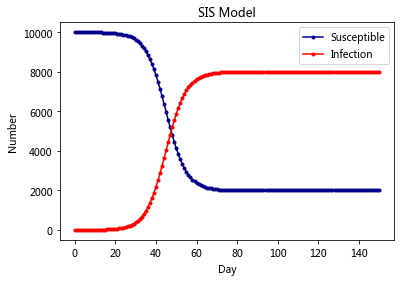
The SIS Model#
Another extension of the SI model is the one that allows for reinfection.
Given S + I = 1, the differential equations have the solution:
The constant \(C = \frac{\beta x_0}{\beta - \gamma - \beta x_0}\)
# N为人群总数
N = 10000
# β为传染率系数
beta = 0.25
# gamma为恢复率系数
gamma = 0.05
# I_0为感染者的初始人数
I_0 = 1
# S_0为易感者的初始人数
S_0 = N - I_0
# T为传播时间
T = 150

# INI为初始状态下的数组
INI = (S_0,I_0)
def funcSIS(inivalue,_):
    Y = np.zeros(2)
    X = inivalue
    # 易感个体变化
    Y[0] = - (beta * X[0]) / N * X[1] + gamma * X[1]
    # 感染个体变化
    Y[1] = (beta * X[0] * X[1]) / N - gamma * X[1]
    return Y

T_range = np.arange(0,T + 1)
RES = spi.odeint(funcSIS,INI,T_range)
plt.plot(RES[:,0],color = 'darkblue',label = 'Susceptible',marker = '.')
plt.plot(RES[:,1],color = 'red',label = 'Infection',marker = '.')
plt.title('SIS Model')
plt.legend()
plt.xlabel('Day')
plt.ylabel('Number')
plt.show()
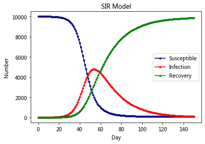
The SIR Model#
For many diseases, there is usually a status of recovery denoted by \(R\). Let \(\gamma\) denote the removal or recovery rate.

However, the differential equations above could not be analytically solved.
# N为人群总数
N = 10000
# β为传染率系数
beta = 0.25
# gamma为恢复率系数
gamma = 0.05
# I_0为感染者的初始人数
I_0 = 1
# R_0为治愈者的初始人数
R_0 = 0
# S_0为易感者的初始人数
S_0 = N - I_0 - R_0
# T为传播时间
T = 150

# INI为初始状态下的数组
INI = (S_0,I_0,R_0)
def funcSIR(inivalue,_):
    Y = np.zeros(3)
    X = inivalue
    # 易感个体变化
    Y[0] = - (beta * X[0] * X[1]) / N
    # 感染个体变化
    Y[1] = (beta * X[0] * X[1]) / N - gamma * X[1]
    # 治愈个体变化
    Y[2] = gamma * X[1]
    return Y

T_range = np.arange(0,T + 1)
RES = spi.odeint(funcSIR,INI,T_range)
plt.plot(RES[:,0],color = 'darkblue',label = 'Susceptible',marker = '.')
plt.plot(RES[:,1],color = 'red',label = 'Infection',marker = '.')
plt.plot(RES[:,2],color = 'green',label = 'Recovery',marker = '.')
plt.title('SIR Model')
plt.legend()
plt.xlabel('Day')
plt.ylabel('Number')
plt.show()
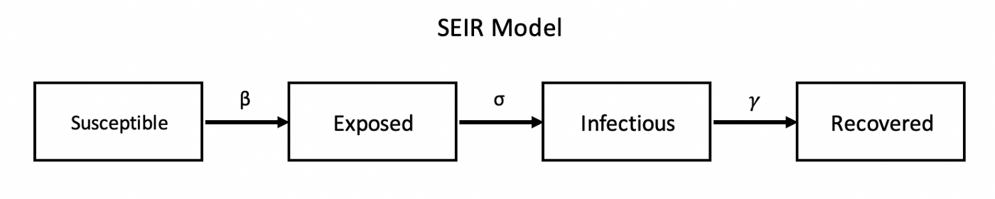
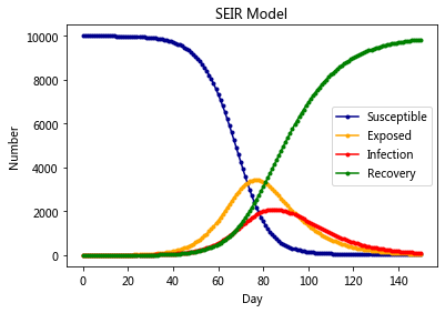
The SEIR Model#
# N为人群总数
N = 10000
# β为传染率系数
beta = 0.6
# gamma为恢复率系数
gamma = 0.1
# Te为疾病潜伏期
Te = 14
# I_0为感染者的初始人数
I_0 = 1
# E_0为潜伏者的初始人数
E_0 = 0
# R_0为治愈者的初始人数
R_0 = 0
# S_0为易感者的初始人数
S_0 = N - I_0 - E_0 - R_0
# T为传播时间
T = 150
# INI为初始状态下的数组
INI = (S_0,E_0,I_0,R_0)
def funcSEIR(inivalue,_):
    Y = np.zeros(4)
    X = inivalue
    # 易感个体变化
    Y[0] = - (beta * X[0] * X[2]) / N
    # 潜伏个体变化
    Y[1] = (beta * X[0] * X[2]) / N - X[1] / Te
    # 感染个体变化
    Y[2] = X[1] / Te - gamma * X[2]
    # 治愈个体变化
    Y[3] = gamma * X[2]
    return Y

T_range = np.arange(0,T + 1)
RES = spi.odeint(funcSEIR,INI,T_range)
plt.plot(RES[:,0],color = 'darkblue',label = 'Susceptible',marker = '.')
plt.plot(RES[:,1],color = 'orange',label = 'Exposed',marker = '.')
plt.plot(RES[:,2],color = 'red',label = 'Infection',marker = '.')
plt.plot(RES[:,3],color = 'green',label = 'Recovery',marker = '.')

plt.title('SEIR Model')
plt.legend()
plt.xlabel('Day')
plt.ylabel('Number')
plt.show()
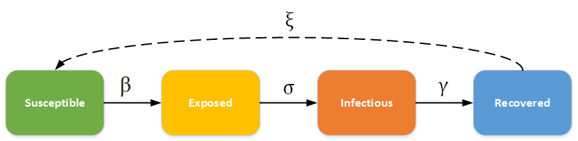
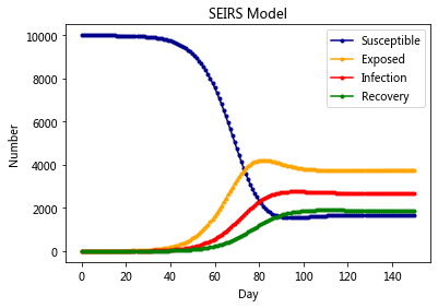
The SEIRS Model#
# N为人群总数
N = 10000
# β为传染率系数
beta = 0.6
# gamma为恢复率系数
gamma = 0.1
# Ts为抗体持续时间
Ts = 7
# Te为疾病潜伏期
Te = 14
# I_0为感染者的初始人数
I_0 = 1
# E_0为潜伏者的初始人数
E_0 = 0
# R_0为治愈者的初始人数
R_0 = 0
# S_0为易感者的初始人数
S_0 = N - I_0 - E_0 - R_0
# T为传播时间
T = 150
# INI为初始状态下的数组
INI = (S_0,E_0,I_0,R_0)


def funcSEIRS(inivalue,_):
    Y = np.zeros(4)
    X = inivalue
    # 易感个体变化
    Y[0] = - (beta * X[0] * X[2]) / N + X[3] / Ts
    # 潜伏个体变化
    Y[1] = (beta * X[0] * X[2]) / N - X[1] / Te
    # 感染个体变化
    Y[2] = X[1] / Te - gamma * X[2]
    # 治愈个体变化
    Y[3] = gamma * X[2] - X[3] / Ts
    return Y

T_range = np.arange(0,T + 1)

RES = spi.odeint(funcSEIRS,INI,T_range)
plt.plot(RES[:,0],color = 'darkblue',label = 'Susceptible',marker = '.')
plt.plot(RES[:,1],color = 'orange',label = 'Exposed',marker = '.')
plt.plot(RES[:,2],color = 'red',label = 'Infection',marker = '.')
plt.plot(RES[:,3],color = 'green',label = 'Recovery',marker = '.')

plt.title('SEIRS Model')
plt.legend()
plt.xlabel('Day')
plt.ylabel('Number')
plt.show()
# https://zhuanlan.zhihu.com/p/115869172
import scipy.integrate as spi
import numpy as np
import matplotlib.pyplot as plt
# N为人群总数
N =11000000
# β为传染率系数
beta = 0.01
# gamma为恢复率系数
gamma = 0.1
#δ为受到治疗系数
δ = 0.3
# Te为疾病潜伏期
Te = 5
# I_0为感染未住院的初始人数
I_0 = 4058
# E_0为潜伏者的初始人数
E_0 = 3178
# R_0为治愈者的初始人数
R_0 = 91750
#T_0为治疗中的初始人数
T_0 = 53941
# S_0为易感者的初始人数
S_0 = N - I_0 - E_0 - R_0 - T_0
# T为传播时间
T = 100
# INI为初始状态下的数组
INI = (S_0,E_0,I_0,R_0,T_0)
def funcSEIR(inivalue,_):
Y = np.zeros(5)
X = inivalue
# 易感个体变化
Y[0] = - (beta * X[0] *( X[2]+X[1])) / N
# 潜伏个体变化
Y[1] = (beta * X[0] *( X[2]+X[1])) / N - X[1] / Te
# 感染未住院
Y[2] = X[1] / Te - δ * X[2]
# 治愈个体变化
Y[3] = gamma * X[4]
#治疗中个体变化
Y[4] = δ* X[2] - gamma* X[4]
return Y
T_range = np.arange(0,T + 1)
RES = spi.odeint(funcSEIR,INI,T_range)
plt.figure(figsize = [8, 8])
plt.subplot(221)
plt.plot(RES[:,0],color = 'darkblue',label = 'Susceptible',marker = '.')
plt.yscale('log')
plt.xscale('log')
plt.legend()
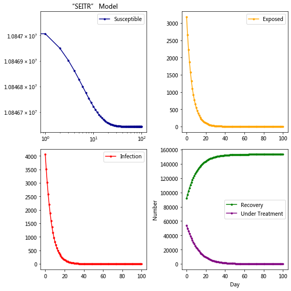
plt.title('“SEITR” Model')
plt.subplot(222)
plt.plot(RES[:,1],color = 'orange',label = 'Exposed',marker = '.')
plt.legend()
plt.subplot(223)
plt.plot(RES[:,2],color = 'red',label = 'Infection',marker = '.')
plt.legend()
plt.subplot(224)
plt.plot(RES[:,3],color = 'green',label = 'Recovery',marker = '.')
plt.plot(RES[:,4],color = 'purple',label = 'Under Treatment',marker = '.')
plt.legend()
plt.xlabel('Day')
plt.ylabel('Number')
plt.tight_layout()
Install#
pip install ndlib
Requirement already satisfied: ndlib in /opt/anaconda3/lib/python3.7/site-packages (5.0.2)
Requirement already satisfied: python-igraph in /opt/anaconda3/lib/python3.7/site-packages (from ndlib) (0.8.2)
Requirement already satisfied: bokeh in /opt/anaconda3/lib/python3.7/site-packages (from ndlib) (1.4.0)
Requirement already satisfied: netdispatch in /opt/anaconda3/lib/python3.7/site-packages (from ndlib) (0.0.5)
Requirement already satisfied: numpy in /opt/anaconda3/lib/python3.7/site-packages (from ndlib) (1.18.1)
Requirement already satisfied: dynetx in /opt/anaconda3/lib/python3.7/site-packages (from ndlib) (0.2.3)
Requirement already satisfied: scipy in /opt/anaconda3/lib/python3.7/site-packages (from ndlib) (1.4.1)
Requirement already satisfied: networkx in /opt/anaconda3/lib/python3.7/site-packages (from ndlib) (2.4)
Requirement already satisfied: future in /opt/anaconda3/lib/python3.7/site-packages (from ndlib) (0.18.2)
Requirement already satisfied: texttable>=1.6.2 in /opt/anaconda3/lib/python3.7/site-packages (from python-igraph->ndlib) (1.6.2)
Requirement already satisfied: Jinja2>=2.7 in /opt/anaconda3/lib/python3.7/site-packages (from bokeh->ndlib) (2.11.1)
Requirement already satisfied: python-dateutil>=2.1 in /opt/anaconda3/lib/python3.7/site-packages (from bokeh->ndlib) (2.8.1)
Requirement already satisfied: tornado>=4.3 in /opt/anaconda3/lib/python3.7/site-packages (from bokeh->ndlib) (6.0.3)
Requirement already satisfied: pillow>=4.0 in /opt/anaconda3/lib/python3.7/site-packages (from bokeh->ndlib) (7.0.0)
Requirement already satisfied: packaging>=16.8 in /opt/anaconda3/lib/python3.7/site-packages (from bokeh->ndlib) (20.1)
Requirement already satisfied: six>=1.5.2 in /opt/anaconda3/lib/python3.7/site-packages (from bokeh->ndlib) (1.14.0)
Requirement already satisfied: PyYAML>=3.10 in /opt/anaconda3/lib/python3.7/site-packages (from bokeh->ndlib) (5.3)
Requirement already satisfied: decorator>=4.3.0 in /opt/anaconda3/lib/python3.7/site-packages (from networkx->ndlib) (4.4.1)
Requirement already satisfied: MarkupSafe>=0.23 in /opt/anaconda3/lib/python3.7/site-packages (from Jinja2>=2.7->bokeh->ndlib) (1.1.1)
Requirement already satisfied: pyparsing>=2.0.2 in /opt/anaconda3/lib/python3.7/site-packages (from packaging>=16.8->bokeh->ndlib) (2.4.6)
Note: you may need to restart the kernel to use updated packages.
Tutorial#
https://ndlib.readthedocs.io/en/latest/tutorial.html
import networkx as nx
import ndlib.models.epidemics as ep
import ndlib.models.ModelConfig as mc
from bokeh.io import output_notebook, show
from ndlib.viz.bokeh.DiffusionTrend import DiffusionTrend
from ndlib.viz.bokeh.DiffusionPrevalence import DiffusionPrevalence
from ndlib.viz.bokeh.MultiPlot import MultiPlot
# Network Definition
g = nx.erdos_renyi_graph(1000, 0.1)
# Model Selection
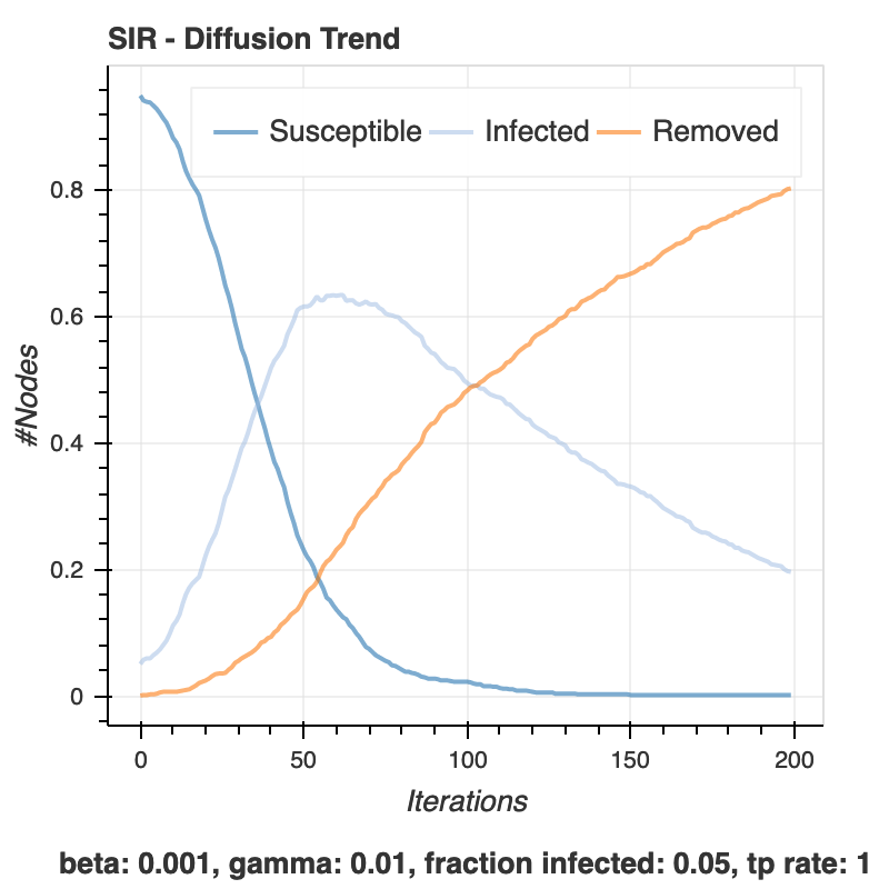
model = ep.SIRModel(g)
# Model Configuration
config = mc.Configuration()
config.add_model_parameter('beta', 0.001)
config.add_model_parameter('gamma', 0.01)
config.add_model_parameter("fraction_infected", 0.05)
model.set_initial_status(config)
# Simulation
iterations = model.iteration_bunch(200)
trends = model.build_trends(iterations)
100%|██████████| 200/200 [00:01<00:00, 183.84it/s]
output_notebook() # show bokeh in notebook
viz = DiffusionTrend(model, trends)
p = viz.plot(width=400, height=400)
show(p)
BokehDeprecationWarning: 'legend' keyword is deprecated, use explicit 'legend_label', 'legend_field', or 'legend_group' keywords instead
BokehDeprecationWarning: 'legend' keyword is deprecated, use explicit 'legend_label', 'legend_field', or 'legend_group' keywords instead
BokehDeprecationWarning: 'legend' keyword is deprecated, use explicit 'legend_label', 'legend_field', or 'legend_group' keywords instead
viz2 = DiffusionPrevalence(model, trends)
p2 = viz2.plot(width=400, height=400)
show(p2)
BokehDeprecationWarning: 'legend' keyword is deprecated, use explicit 'legend_label', 'legend_field', or 'legend_group' keywords instead
BokehDeprecationWarning: 'legend' keyword is deprecated, use explicit 'legend_label', 'legend_field', or 'legend_group' keywords instead
BokehDeprecationWarning: 'legend' keyword is deprecated, use explicit 'legend_label', 'legend_field', or 'legend_group' keywords instead
vm = MultiPlot()
vm.add_plot(p)
vm.add_plot(p2)
m = vm.plot()
show(m)
Kertesz Threshold model#
The Kertesz Threshold model was introduced in 2015 by Ruan et al. [1] and it is an extension of the Watts threshold model [2].
We set the initial infected as well blocked node sets equals to the 10% of the overall population, assign a threshold of 0.25 to all the nodes and impose an probability of spontaneous adoptions of 40%.
[1] Z. Ruan, G. In ̃iguez, M. Karsai, and J. Kertész, “Kinetics of social contagion,” Phys. Rev. Lett., vol. 115, p. 218702, Nov 2015.
[2] D.J. Watts, “A simple model of global cascades on random networks,” Proceedings of the National Academy of Sciences, vol. 99, no. 9, pp. 5766–5771, 2002.
# Network topology
g = nx.erdos_renyi_graph(1000, 0.1)

# Model selection
th_model = ep.KerteszThresholdModel(g)

# Model Configuration
config = mc.Configuration()
config.add_model_parameter('adopter_rate', 0.4)
config.add_model_parameter('percentage_blocked', 0.1)
config.add_model_parameter('fraction_infected', 0.1)

# Setting node parameters
threshold = 0.25
for i in g.nodes():
    config.add_node_configuration("threshold", i, threshold)

th_model.set_initial_status(config)

# Simulation execution
iterations = th_model.iteration_bunch(200)
100%|██████████| 200/200 [00:00<00:00, 207.32it/s]
output_notebook() # show bokeh in notebook

trends = th_model.build_trends(iterations)

viz = DiffusionTrend(th_model, trends)
p = viz.plot(width=400, height=400)
show(p)
BokehDeprecationWarning: 'legend' keyword is deprecated, use explicit 'legend_label', 'legend_field', or 'legend_group' keywords instead
BokehDeprecationWarning: 'legend' keyword is deprecated, use explicit 'legend_label', 'legend_field', or 'legend_group' keywords instead
BokehDeprecationWarning: 'legend' keyword is deprecated, use explicit 'legend_label', 'legend_field', or 'legend_group' keywords instead
viz2 = DiffusionPrevalence(th_model, trends)
p2 = viz2.plot(width=400, height=400)
show(p2)
BokehDeprecationWarning: 'legend' keyword is deprecated, use explicit 'legend_label', 'legend_field', or 'legend_group' keywords instead
BokehDeprecationWarning: 'legend' keyword is deprecated, use explicit 'legend_label', 'legend_field', or 'legend_group' keywords instead
BokehDeprecationWarning: 'legend' keyword is deprecated, use explicit 'legend_label', 'legend_field', or 'legend_group' keywords instead
Model Comparisions#
# model comparisions
vm = MultiPlot()
vm.add_plot(p)

# SIS
sis_model = ep.SISModel(g)
config = mc.Configuration()
config.add_model_parameter('beta', 0.001)
config.add_model_parameter('lambda', 0.01)
config.add_model_parameter("fraction_infected", 0.05)
sis_model.set_initial_status(config)
iterations = sis_model.iteration_bunch(200)
trends = sis_model.build_trends(iterations)

viz = DiffusionTrend(sis_model, trends)
p3 = viz.plot(width=400, height=400)
vm.add_plot(p3)

# SI
si_model = ep.SIModel(g)
config = mc.Configuration()
config.add_model_parameter('beta', 0.001)
config.add_model_parameter("fraction_infected", 0.05)
si_model.set_initial_status(config)
iterations = si_model.iteration_bunch(200)
trends = si_model.build_trends(iterations)

viz = DiffusionTrend(si_model, trends)
p4 = viz.plot(width=400, height=400)
vm.add_plot(p4)

# Threshold
th_model = ep.ThresholdModel(g)
config = mc.Configuration()

# Set individual node threshold
threshold = 0.40
for n in g.nodes():
    config.add_node_configuration("threshold", n, threshold)

config.add_model_parameter("fraction_infected", 0.30)
th_model.set_initial_status(config)
iterations = th_model.iteration_bunch(60)
trends = th_model.build_trends(iterations)

viz = DiffusionTrend(th_model, trends)
p5 = viz.plot(width=400, height=400)
vm.add_plot(p5)

m = vm.plot()
show(m)
100%|██████████| 200/200 [00:01<00:00, 149.48it/s]
BokehDeprecationWarning: 'legend' keyword is deprecated, use explicit 'legend_label', 'legend_field', or 'legend_group' keywords instead
BokehDeprecationWarning: 'legend' keyword is deprecated, use explicit 'legend_label', 'legend_field', or 'legend_group' keywords instead
100%|██████████| 200/200 [00:01<00:00, 198.91it/s]
BokehDeprecationWarning: 'legend' keyword is deprecated, use explicit 'legend_label', 'legend_field', or 'legend_group' keywords instead
BokehDeprecationWarning: 'legend' keyword is deprecated, use explicit 'legend_label', 'legend_field', or 'legend_group' keywords instead
100%|██████████| 60/60 [00:00<00:00, 94.43it/s]
BokehDeprecationWarning: 'legend' keyword is deprecated, use explicit 'legend_label', 'legend_field', or 'legend_group' keywords instead
BokehDeprecationWarning: 'legend' keyword is deprecated, use explicit 'legend_label', 'legend_field', or 'legend_group' keywords instead
Threshold model#
The threshold model was introduced in 1978 by Granovetter [1]. A node has two distinct and mutually exclusive behavioral alternatives, e.g., the decision to do or not do something. Individual decision depends on the percentage of its neighbors have made the same choice, thus imposing a threshold.
each node has its own threshold;
during a generic iteration every node is observed:
if the percentage of its infected neighbors is grater than its threshold it becomes infected as well.
Granovetter, “Threshold models of collective behavior,” The American Journal of Sociology, vol. 83, no. 6, pp. 1420–1443, 1978.

import networkx as nx
import ndlib.models.ModelConfig as mc
import ndlib.models.epidemics as ep

def watts_model_ba_network(m, threshold, fraction_infected, iteration_num):
    # change these two parameters
    # num_neighbors = 1
    # threshold = 0.5
    # fraction_infected = 0.1
    # iteration_num = 30

    # Network topology
    #g = nx.erdos_renyi_graph(1000, 0.1)
    g = nx.barabasi_albert_graph(1000, m)
    # Model selection
    model = ep.ThresholdModel(g)
    # Model Configuration
    config = mc.Configuration()
    config.add_model_parameter('fraction_infected', fraction_infected)
    # Setting node parameters
    for i in g.nodes():
        config.add_node_configuration("threshold", i, threshold)

    model.set_initial_status(config)
    # Simulation execution
    iterations = model.iteration_bunch(iteration_num)
    return model, iterations
def plot_diffusion(model, iterations):
    output_notebook() # show bokeh in notebook
    trends = model.build_trends(iterations)
    viz = DiffusionTrend(model, trends)
    p = viz.plot(width=400, height=400)

    viz2 = DiffusionPrevalence(model, trends)
    p2 = viz2.plot(width=400, height=400)

    vm = MultiPlot()
    vm.add_plot(p)
    vm.add_plot(p2)
    m = vm.plot()
    show(m)
model, iterations = watts_model_ba_network(1, 0.5, 0.1, 30)
plot_diffusion(model, iterations)
100%|██████████| 30/30 [00:00<00:00, 465.02it/s]
BokehDeprecationWarning: 'legend' keyword is deprecated, use explicit 'legend_label', 'legend_field', or 'legend_group' keywords instead
BokehDeprecationWarning: 'legend' keyword is deprecated, use explicit 'legend_label', 'legend_field', or 'legend_group' keywords instead
BokehDeprecationWarning: 'legend' keyword is deprecated, use explicit 'legend_label', 'legend_field', or 'legend_group' keywords instead
BokehDeprecationWarning: 'legend' keyword is deprecated, use explicit 'legend_label', 'legend_field', or 'legend_group' keywords instead
model, iterations = watts_model_ba_network(5, 0.5, 0.1, 30)
plot_diffusion(model, iterations)
100%|██████████| 30/30 [00:00<00:00, 308.63it/s]
BokehDeprecationWarning: 'legend' keyword is deprecated, use explicit 'legend_label', 'legend_field', or 'legend_group' keywords instead
BokehDeprecationWarning: 'legend' keyword is deprecated, use explicit 'legend_label', 'legend_field', or 'legend_group' keywords instead
BokehDeprecationWarning: 'legend' keyword is deprecated, use explicit 'legend_label', 'legend_field', or 'legend_group' keywords instead
BokehDeprecationWarning: 'legend' keyword is deprecated, use explicit 'legend_label', 'legend_field', or 'legend_group' keywords instead
model, iterations = watts_model_ba_network(2, 0.2, 0.1, 30)
plot_diffusion(model, iterations)
100%|██████████| 30/30 [00:00<00:00, 1237.37it/s]
BokehDeprecationWarning: 'legend' keyword is deprecated, use explicit 'legend_label', 'legend_field', or 'legend_group' keywords instead
BokehDeprecationWarning: 'legend' keyword is deprecated, use explicit 'legend_label', 'legend_field', or 'legend_group' keywords instead
BokehDeprecationWarning: 'legend' keyword is deprecated, use explicit 'legend_label', 'legend_field', or 'legend_group' keywords instead
BokehDeprecationWarning: 'legend' keyword is deprecated, use explicit 'legend_label', 'legend_field', or 'legend_group' keywords instead
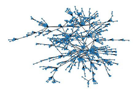
nx.draw(g, node_size = 10)
General Threshold#
The General Threshold model was introduced in 2003 by Kempe [1].
In this model, during an epidemics, a node is allowed to change its status from Susceptible to Infected.
At time t nodes become Infected if the sum of the weight of the infected neighbors is greater than the threshold
David Kempe , Jon Kleinberg, and Éva Tardos. “Maximizing the spread of influence through a social network.” Proceedings of the ninth ACM SIGKDD international conference on Knowledge discovery and data mining. ACM, 2003.
https://ndlib.readthedocs.io/en/latest/reference/models/epidemics/GeneralThreshold.html
Generalised Threshold#
It was introduced in 2017 by Török and Kertesz [1]. In this model, a node is allowed to change its status from Susceptible to Infected. The model is instantiated on a graph having a non-empty set of infected nodes.
At time
tnodes become Infected with ratemu t/tauNodes for which the ratio of the active friends dropped below the threshold are moved to the Infected queue
Nodes in the Infected queue become infected with rate tau. If this happens check all its friends for threshold
János Török and János Kertész “Cascading collapse of online social networks” Scientific reports, vol. 7 no. 1, 2017
https://ndlib.readthedocs.io/en/latest/reference/models/epidemics/GeneralisedThreshold.html